Python new magic method explained

2019-12-27

A good LinkedIn profile checklist

2020-04-26

RCNN, Fast RCNN, and faster RCNN algorithms for Object Detection Explained

1. A Simple Way of Solving an Object Detection Task (using Deep Learning)

The below image is a popular example of illustrating how an object detection algorithm works. Each object in the image, from a person to a kite, has been located and identified with a certain level of precision.

Let’s start with the simplest deep learning approach, and a widely used one, for detecting objects in images – Convolutional Neural Networks or CNNs. If your understanding of CNNs is a little rusty, I recommend going through this article first.

But I’ll briefly summarize the inner workings of a CNN for you. Take a look at the below image:

We pass an image to the network, and it is then sent through various convolutions and pooling layers. Finally, we get the output in the form of the object’s class. Fairly straightforward, isn’t it?

For each input image, we get a corresponding class as an output. Can we use this technique to detect various objects in an image? Yes, we can! Let’s look at how we can solve a general object detection problem using CNN.

1. First, we take an image as input:

2. Then we divide the image into various regions:

3. We will then consider each region as a separate image.
4. Pass all these regions (images) to the CNN and classify them into various classes.
5. Once we have divided each region into its corresponding class, we can combine all these regions to get the original image with the detected objects:

The problem with using this approach is that the objects in the image can have different aspect ratios and spatial locations. For instance, in some cases, the object might be covering most of the image, while in others the object might only be covering a small percentage of the image. The shapes of the objects might also be different (which happens a lot in real-life use cases).

As a result of these factors, we would require a very large number of regions resulting in a huge amount of computational time. So to solve this problem and reduce the number of regions, we can use region-based CNN, which selects the regions using a proposal method. Let’s understand what this region-based CNN can do for us.

2. Understanding Region-Based Convolutional Neural Network

2.1 Intuition of RCNN

Instead of working on a massive number of regions, the RCNN algorithm proposes a bunch of boxes in the image and checks if any of these boxes contain any object. RCNN uses selective search to extract these boxes from an image (these boxes are called regions).

Let’s first understand what selective search is and how it identifies the different regions. There are basically four regions that form an object: varying scales, colors, textures, and enclosure. The selective search identifies these patterns in the image and based on that, proposes various regions. Here is a brief overview of how selective search works:

It first takes an image as input:

Then, it generates initial sub-segmentations so that we have multiple regions from this image:

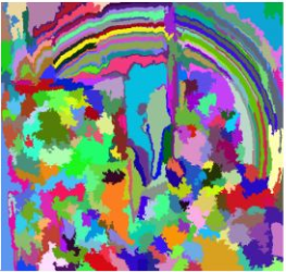
The technique then combines the similar regions to form a larger region (based on color similarity, texture similarity, size similarity, and shape compatibility):

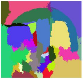
Finally, these regions then produce the final object locations (Region of Interest).

Below is a succinct summary of the steps followed in RCNN to detect objects:

We first take a pre-trained convolutional neural network.
Then, this model is retrained. We train the last layer of the network based on the number of classes that need to be detected.
The third step is to get the Region of Interest for each image. We then reshape all these regions so that they can match the CNN input size.
After getting the regions, we train SVM to classify objects and backgrounds. For each class, we train one binary SVM.
Finally, we train a linear regression model to generate tighter bounding boxes for each identified object in the image.

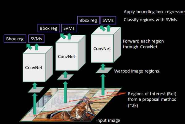
You might get a better idea of the above steps with a visual example (Images for the example shown below are taken from this paper). So let’s take one!

First, an image is taken as an input:

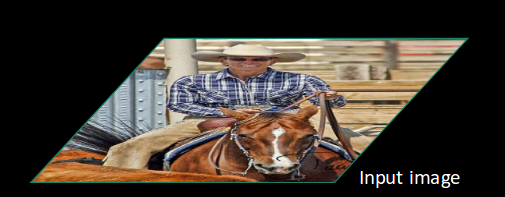
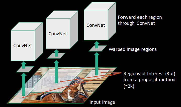
Then, we get the Regions of Interest (ROI) using some proposal method (for example, selective search as seen above):

All these regions are then reshaped as per the input of the CNN, and each region is passed to the ConvNet:

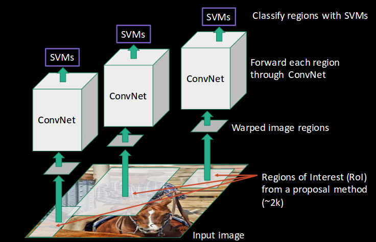
CNN then extracts features for each region and SVMs are used to divide these regions into different classes:

Finally, a bounding box regression (Bbox reg) is used to predict the bounding boxes for each identified region:

And this, in a nutshell, is how an RCNN helps us to detect objects.

2.2 Problems with RCNN

So far, we’ve seen how RCNN can be helpful for object detection. But this technique comes with its own limitations. Training an RCNN model is expensive and slow thanks to the below steps:

Extracting 2,000 regions for each image based on selective search
Extracting features using CNN for every image region. Suppose we have N images, then the number of CNN features will be N*2,000
The entire process of object detection using RCNN has three models:
1. CNN for feature extraction
2. Linear SVM classifier for identifying objects
3. Regression model for tightening the bounding boxes.

All these processes combine to make RCNN very slow. It takes around 40-50 seconds to make predictions for each new image, which essentially makes the model cumbersome and practically impossible to build when faced with a gigantic dataset. Here’s the good news – we have another object detection technique that fixes most of the limitations we saw in RCNN.

3. Understanding Fast RCNN

3.1 Intuition of Fast RCNN

What else can we do to reduce the computation time an RCNN algorithm typically takes? Instead of running a CNN 2,000 times per image, we can run it just once per image and get all the regions of interest (regions containing some object).

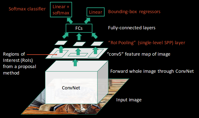
Ross Girshick, the author of RCNN, came up with the idea of running the CNN just once per image and then finding a way to share that computation across the 2,000 regions. In Fast RCNN, we feed the input image to the CNN, which in turn generates the convolutional feature maps. Using these maps, the regions of proposals are extracted. We then use an RoI pooling layer to reshape all the proposed regions into a fixed size, so that they can be fed into a fully connected network.

Let’s break this down into steps to simplify the concept:

As with the earlier two techniques, we take an image as input.
This image is passed to a ConvNet which in turn generates the Regions of Interest.
An RoI pooling layer is applied to all of these regions to reshape them as per the input of the ConvNet. Then, each region is passed on to a fully connected network.
A softmax layer is used on top of the fully connected network to output classes. Along with the softmax layer, a linear regression layer is also used parallel to output bounding box coordinates for predicted classes.

So, instead of using three different models (like in RCNN), Fast RCNN uses a single model which extracts features from the regions, divides them into different classes, and returns the boundary boxes for the identified classes simultaneously.

To break this down even further, I’ll visualize each step to add a practical angle to the explanation.

We follow the now well-known step of taking an image as input:

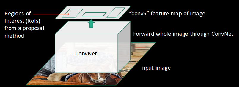
This image is passed to a ConvNet which returns the region of interests accordingly:

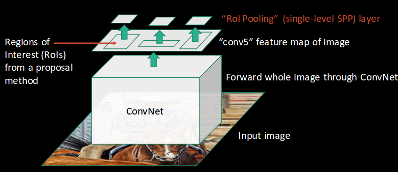
Then we apply the RoI pooling layer to the extracted regions of interest to make sure all the regions are of the same size:

Finally, these regions are passed on to a fully connected network which classifies them, as well as returns the bounding boxes using softmax and linear regression layers simultaneously:

This is how Fast RCNN resolves two major issues of RCNN, i.e., passing one instead of 2,000 regions per image to the ConvNet, and using one instead of three different models for extracting features, classification, and generating bounding boxes.

3.2 Problems with Fast RCNN

But even Fast RCNN has certain problem areas. It also uses selective search as a proposed method to find the Regions of Interest, which is a slow and time-consuming process. It takes around 2 seconds per image to detect objects, which is much better compared to RCNN. But when we consider large real-life datasets, then even a Fast RCNN doesn’t look so fast anymore.

But there’s yet another object detection algorithm that trumps Fast RCNN. And something tells me you won’t be surprised by its name.

4. Understanding Faster RCNN

4.1. Intuition of Faster RCNN

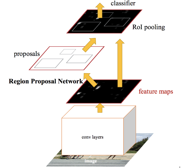
Faster RCNN is the modified version of Fast RCNN. The major difference between them is that Fast RCNN uses the selective search for generating Regions of Interest, while Faster RCNN uses “Region Proposal Network”, aka RPN. RPN takes image feature maps as input and generates a set of object proposals, each with an objectness score as output.

The below steps are typically followed in a Faster RCNN approach:

We take an image as input and pass it to the ConvNet which returns the feature map for that image.
Region proposal network is applied on these feature maps. This returns the object proposals along with their objectness score.
An RoI pooling layer is applied to these proposals to bring down all the proposals to the same size.
Finally, the proposals are passed to a fully connected layer which has a softmax layer and a linear regression layer at its top, to classify and output the bounding boxes for objects.

Let me briefly explain how this Region Proposal Network (RPN) actually works.

To begin with, Faster RCNN takes the feature maps from CNN and passes them on to the Region Proposal Network. RPN uses a sliding window over these feature maps, and at each window, it generates k Anchor boxes of different shapes and sizes:

Anchor boxes are fixed-sized boundary boxes that are placed throughout the image and have different shapes and sizes. For each anchor, RPN predicts two things:

The first is the probability that an anchor is an object (it does not consider which class the object belongs to)
Second is the bounding box regressor for adjusting the anchors to better fit the object

We now have bounding boxes of different shapes and sizes which are passed on to the RoI pooling layer. Now it might be possible that after the RPN step, there are proposals with no classes assigned to them. We can take each proposal and crop it so that each proposal contains an object. This is what the RoI pooling layer does. It extracts fixed sized feature maps for each anchor:

Then these feature maps are passed to a fully connected layer which has a softmax and a linear regression layer. It finally classifies the object and predicts the bounding boxes for the identified objects.

4.2 Problems with Faster RCNN

All of the object detection algorithms we have discussed so far use regions to identify the objects. The network does not look at the complete image in one go but focuses on parts of the image sequentially. This creates two complications:

The algorithm requires many passes through a single image to extract all the objects
As different systems are working one after the other, the performance of the systems further ahead depends on how the previous systems performed

5. Summary of the Algorithms covered

Let’s quickly summarize the different algorithms in the R-CNN family (R-CNN, Fast R-CNN, and Faster R-CNN) that we saw in the first article. This will help lay the ground for our implementation part later when we will predict the bounding boxes present in previously unseen images (new data).

R-CNN extracts a bunch of regions from the given image using selective search and then checks if any of these boxes contains an object. We first extract these regions, and for each region, CNN is used to extract specific features. Finally, these features are then used to detect objects. Unfortunately, R-CNN becomes rather slow due to the multiple steps involved in the process.

R-CNN

Fast R-CNN, on the other hand, passes the entire image to ConvNet which generates regions of interest (instead of passing the extracted regions from the image). Also, instead of using three different models (as we saw in R-CNN), it uses a single model which extracts features from the regions, classifies them into different classes, and returns the bounding boxes.

All these steps are done simultaneously, thus making it execute faster as compared to R-CNN. Fast R-CNN is, however, not fast enough when applied on a large dataset as it also uses selective search for extracting the regions.

Fast R-CNN

Faster R-CNN fixes the problem of selective search by replacing it with Region Proposal Network (RPN). We first extract feature maps from the input image using ConvNet and then pass those maps through a RPN which returns object proposals. Finally, these maps are classified and the bounding boxes are predicted.

Faster R-CNN

I have summarized below the steps followed by a Faster R-CNN algorithm to detect objects in an image:

Take an input image and pass it to the ConvNet which returns feature maps for the image
Apply Region Proposal Network (RPN) on these feature maps and get object proposals
Apply ROI pooling layer to bring down all the proposals to the same size
Finally, pass these proposals to a fully connected layer in order to classify any predict the bounding boxes for the image

The below table is a nice summary of all the algorithms we have covered in this post.

Algorithm	Features	Prediction time / image	Limitations
CNN	Divides the image into multiple regions and then classifies each region into various classes.	–	Needs a lot of regions to predict accurately and hence high computation time.
RCNN	Uses selective search to generate regions. Extracts around 2000 regions from each image.	40-50 seconds	High computation time as each region is passed to the CNN separately also it uses three different models for making predictions.
Fast RCNN	Each image is passed only once to the CNN and feature maps are extracted. Selective search is used on these maps to generate predictions. Combines all the three models used in RCNN together.	2 seconds	Selective search is slow and hence computation time is still high.
Faster RCNN	Replaces the selective search method with the region proposal network which made the algorithm much faster.	0.2 seconds	Object proposal takes time and as there are different systems working one after the other, the performance of systems depends on how the previous system has performed.

6. Real-world object detection example using Faster R-CNN

Now that we have a grasp on this topic, it’s time to jump from the theory into the practical part of our article. Let’s implement Faster R-CNN using a really cool (and rather useful) dataset with potential real-life applications!

Understanding the Problem Statement

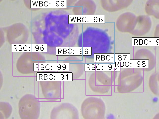
We will be working on a healthcare-related dataset and the aim here is to solve a Blood Cell Detection problem. Our task is to detect all the Red Blood Cells (RBCs), White Blood Cells (WBCs), and Platelets in each image taken via microscopic image readings. Below is a sample of what our final predictions should look like:

The reason for choosing this dataset is that the density of RBCs, WBCs, and Platelets in our bloodstream provides a lot of information about the immune system and hemoglobin. This can help us potentially identify whether a person is healthy or not, and if any discrepancy is found in their blood, actions can be taken quickly to diagnose that.

Manually looking at the sample via a microscope is a tedious process. And this is where Deep Learning models play such a vital role. They can classify and detect blood cells from microscopic images with impressive precision.

The full blood cell detection dataset for our challenge can be downloaded from here. I have modified the data a tiny bit for the scope of this article:

The bounding boxes have been converted from the given .xml format to a .csv format
I have also created the training and test set split on the entire dataset by randomly picking images for the split

Note that we will be using the popular Keras framework with a TensorFlow backend in Python to train and build our model.

Setting up the System

Before we actually get into the model building phase, we need to ensure that the right libraries and frameworks have been installed. The below libraries are required to run this project:

pandas
matplotlib
tensorflow (keras– 2.0.3)
numpy
opencv-python
sklearn
h5py

Most of the above-mentioned libraries will already be present on your machine if you have Anaconda and Jupyter Notebooks installed. Additionally, I recommend downloading the requirement.txt file from this link and using that to install the remaining libraries. Type the following command in the terminal to do this:

pip install -r requirement.txt

Alright, our system is now set and we can move on to working with the data!

Data Exploration

It’s always a good idea (and frankly, a mandatory step) to first explore the data we have. This helps us not only unearth hidden patterns but gain valuable overall insight into what we are working with. The three files I have created out of the entire dataset are:

train_images: Images that we will be using to train the model. We have the classes and the actual bounding boxes for each class in this folder.
test_images: Images in this folder will be used to make predictions using the trained model. This set is missing the classes and the bounding boxes for these classes.
train.csv: Contains the name, class, and bounding box coordinates for each image. There can be multiple rows for one image as a single image can have more than one object.

Let’s read the .csv file (you can create your own .csv file from the original dataset if you feel like experimenting) and print out the first few rows. We’ll need to first import the below libraries for this:

# importing required libraries
import pandas as pd
import matplotlib.pyplot as plt
%matplotlib inline
from matplotlib import patches

# read the csv file using read_csv function of pandas
train = pd.read_csv("train.csv")
train.head()

There are 6 columns in the train file. Let’s understand what each column represents:

image_names: contains the name of the image
cell_type: denotes the type of the cell
xmin: x-coordinate of the bottom-left part of the image
xmax: x-coordinate of the top right part of the image
ymin: y-coordinate of the bottom-left part of the image
ymax: y-coordinate of the top right part of the image

Let’s now print an image to visualize what we’re working with:

# reading single image using imread function of matplotlib
image = plt.imread('images/1.jpg')
plt.imshow(image)

This is what a blood cell image looks like. Here, the blue part represents the WBCs, and the slightly red parts represent the RBCs. Let’s look at how many images, and the different types of classes, there are in our training set.

# Number of unique training images
train['image_names'].nunique()

So, we have 254 training images.

# Number of classes
train['cell_type'].value_counts()

We have three different classes of cells, i.e., RBC, WBC, and Platelets. Finally, let’s look at what an image with detected objects will look like:

fig = plt.figure()

#add axes to the image
ax = fig.add_axes([0,0,1,1])

# read and plot the image
image = plt.imread('images/1.jpg')
plt.imshow(image)

# iterating over the image for different objects
for _,row in train[train.image_names == "1.jpg"].iterrows():
    xmin = row.xmin
    xmax = row.xmax
    ymin = row.ymin
    ymax = row.ymax
    
    width = xmax - xmin
    height = ymax - ymin
    
    # assign different color to different classes of objects
    if row.cell_type == 'RBC':
        edgecolor = 'r'
        ax.annotate('RBC', xy=(xmax-40,ymin+20))
    elif row.cell_type == 'WBC':
        edgecolor = 'b'
        ax.annotate('WBC', xy=(xmax-40,ymin+20))
    elif row.cell_type == 'Platelets':
        edgecolor = 'g'
        ax.annotate('Platelets', xy=(xmax-40,ymin+20))
        
    # add bounding boxes to the image
    rect = patches.Rectangle((xmin,ymin), width, height, edgecolor = edgecolor, facecolor = 'none')
    
    ax.add_patch(rect)

This is what a training example looks like. We have the different classes and their corresponding bounding boxes. Let’s now train our model on these images. We will be using the keras_frcnn library to train our model as well as to get predictions on the test images.

Implementing Faster R-CNN

For implementing the Faster R-CNN algorithm, we will be following the steps mentioned in this Github repository. So as the first step, make sure you clone this repository. Open a new terminal window and type the following to do this:

git clone https://github.com/kbardool/keras-frcnn.git

Move the train_images and test_images folder, as well as the train.csv file, to the cloned repository. In order to train the model on a new dataset, the format of the input should be:

filepath,x1,y1,x2,y2,class_name

where,

filepath is the path of the training image
x1 is the xmin coordinate for the bounding box
y1 is the ymin coordinate for the bounding box
x2 is the xmax coordinate for the bounding box
y2 is the ymax coordinate for the bounding box
class_name is the name of the class in that bounding box

We need to convert the .csv format into a .txt file which will have the same format as described above. Make a new dataframe, fill all the values as per the format into that dataframe, and then save it as a .txt file.

data = pd.DataFrame()
data['format'] = train['image_names']

# as the images are in train_images folder, add train_images before the image name
for i in range(data.shape[0]):
    data['format'][i] = 'train_images/' + data['format'][i]

# add xmin, ymin, xmax, ymax and class as per the format required
for i in range(data.shape[0]):
    data['format'][i] = data['format'][i] + ',' + str(train['xmin'][i]) + ',' + str(train['ymin'][i]) + ',' + str(train['xmax'][i]) + ',' + str(train['ymax'][i]) + ',' + train['cell_type'][i]

data.to_csv('annotate.txt', header=None, index=None, sep=' ')

What’s next?

Train our model! We will be using the train_frcnn.py file to train the model.

cd keras-frcnn
python train_frcnn.py -o simple -p annotate.txt

It will take a while to train the model due to the size of the data. If possible, you can use a GPU to make the training phase faster. You can also try to reduce the number of epochs as an alternate option. To change the number of epochs, go to the train_frcnn.py file in the cloned repository and change the num_epochs parameter accordingly.

Every time the model sees an improvement, the weights of that particular epoch will be saved in the same directory as “model_frcnn.hdf5”. These weights will be used when we make predictions on the test set.

It might take a lot of time to train the model and get the weights, depending on the configuration of your machine. I suggest using the weights I’ve got after training the model for around 500 epochs. You can download these weights from here. Ensure you save these weights in the cloned repository.

So our model has been trained and the weights are set. It’s prediction time! Keras_frcnn makes the predictions for the new images and saves them in a new folder. We just have to make two changes in the test_frcnn.py file to save the images:

Remove the comment from the last line of this file:
cv2.imwrite(‘./results_imgs/{}.png’.format(idx), img)
Add comments on the second last and third last line of this file:
# cv2.imshow(‘img’, img)
# cv2.waitKey(0)

Let’s make the predictions for the new images:

python test_frcnn.py -p test_images

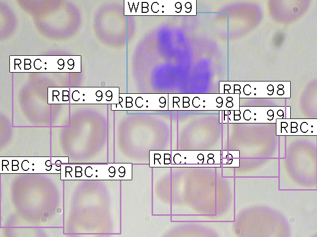
Finally, the images with the detected objects will be saved in the “results_imgs” folder. Below are a few examples of the predictions I got after implementing Faster R-CNN:

Result 1

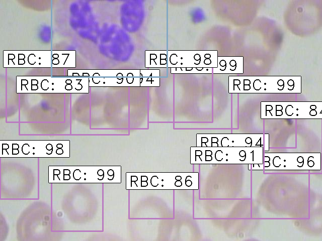
Result 2

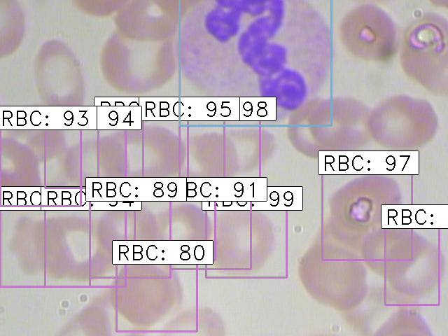
Result 3

Result 4

End Notes

Object detection is a fascinating field and is rightly seeing a ton of traction in commercial, as well as research applications. Thanks to advances in modern hardware and computational resources, breakthroughs in this space have been quick and ground-breaking. R-CNN algorithms have truly been a game-changer for object detection tasks. There has suddenly been a spike in recent years in the amount of computer vision applications being created, and R-CNN is at the heart of most of them. Keras_frcnn proved to be an excellent library for object detection, but there are still more advanced techniques like YOLO, SSD, etc.

References:

https://medium.com/@smallfishbigsea/faster-r-cnn-explained-864d4fb7e3f8

https://engineering.matterport.com/splash-of-color-instance-segmentation-with-mask-r-cnn-and-tensorflow-7c761e238b46

https://towardsdatascience.com/r-cnn-fast-r-cnn-faster-r-cnn-yolo-object-detection-algorithms-36d53571365e

https://blog.athelas.com/a-brief-history-of-cnns-in-image-segmentation-from-r-cnn-to-mask-r-cnn-34ea83205de4

https://cv-tricks.com/object-detection/faster-r-cnn-yolo-ssd/

https://tryolabs.com/blog/2017/08/30/object-detection-an-overview-in-the-age-of-deep-learning/

https://towardsdatascience.com/r-cnn-for-object-detection-a-technical-summary-9e7bfa8a557c

https://towardsdatascience.com/review-faster-r-cnn-object-detection-f5685cb30202

https://towardsdatascience.com/fast-r-cnn-for-object-detection-a-technical-summary-a0ff94faa022

https://medium.com/egen/region-proposal-network-rpn-backbone-of-faster-r-cnn-4a744a38d7f9

https://towardsdatascience.com/deep-learning-for-object-detection-a-comprehensive-review-73930816d8d9