A tutorial on Scikit-Learn Pipeline, ColumnTransformer, and FeatureUnion

2022-08-30

Understand Q-Learning in Reinforcement Learning with a numerical example and Python implementation

2022-09-06

Setup collaborative MLflow with PostgreSQL as Tracking Server and MinIO as Artifact Store using docker containers

Preparing the environment

Note: I have tested the codes on Linux. It can certainly be run on Windows and macOS with small modifications.

Clone the repository, and navigate to the downloaded folder.

git clone https://github.com/iamirmasoud/mlflow_postgres_minio.git
cd mlflow_postgres_minio

Create (and activate) a new environment

conda create -n mlflow_env python=3.7
conda activate mlflow_env

Install the prerequisites for building the psycopg2 package from source on Ubuntu:

sudo apt install libpq-dev python3-dev

Install requirements for the environment:

pip install -r requirements.txt

Setting up a PostgreSQL Database Tracking URI and MinIO Artifact URI

Running PostgreSQL and MinIO containers using Docker Compose

1. Run the following docker-compose command to start a PostgreSQL and a MinIO server:

docker-compose  up -d

Here is the content docker-compose.yml:

version: '3'

services:
  mlflow_postgres:
    image: postgres:13
    container_name: postgres_db
    environment:
      - POSTGRES_USER=postgres
      - POSTGRES_PASSWORD=postgres
      - POSTGRES_DB=mlflow_db
    volumes:
      - postgres_data:/var/lib/postgresql/data
    ports:
      - "5432:5432"
  minio:
    image: minio/minio
    ports:
      - "9000:9000"
      - "9001:9001"
    volumes:
      - minio_data:/data
    environment:
      MINIO_ROOT_USER: masoud
      MINIO_ROOT_PASSWORD: Strong#Pass#2022
    command: server --console-address ":9001" /data
volumes:
  postgres_data: { }
  minio_data: { }

You can run the docker ps command to check if containers were created or not.

3. Verify the new database was created

docker exec -it postgres_db psql -U postgres -c "\l"

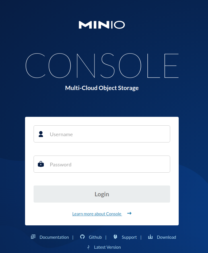
You should be able to access MinIO Console. Open your browser and go to http://127.0.0.1:9001 to open the MinIO Console login page. Log in with the Root User and Root Pass you set in docker-compose.yml file (masoud and Strong#Pass#2022 in my case).

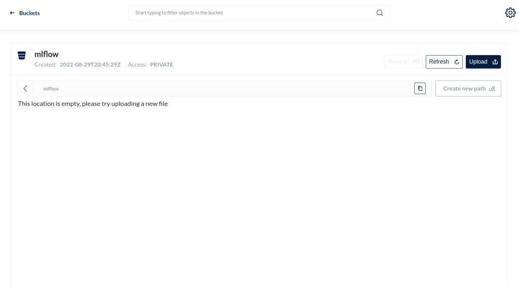
From the MinIO UI, create a bucket called mlflow bucket by clicking on the create bucket button in the bottom right corner.

MLflow Examples

From here you can open the experiment.ipynb and follow along with the codes. Again, I strongly recommend you read this post to become familiar with the basics of MLflow.

Using the Tracking API

In order to use a PostgreSQL DB, we must set a new tracking URI that uses the PostgreSQL DB we configured above. The database is encoded as: <dialect>+<driver>://<username>:<password>@<host>:<port>/<database>. We also must set the S3 endpoint URL with the URL returned when we spun up our MinIO UI. Lastly, our environment must know the Access Key and Secret Key.

import pandas as pd
import numpy as np
from sklearn.metrics import mean_squared_error, mean_absolute_error, r2_score
from sklearn.model_selection import train_test_split
from sklearn.linear_model import ElasticNet
import os
import mlflow
import mlflow.sklearn

os.environ['MLFLOW_TRACKING_URI'] = 'postgresql+psycopg2://postgres:postgres@localhost/mlflow_db'
os.environ['MLFLOW_S3_ENDPOINT_URL'] = "http://127.0.0.1:9000"
os.environ['AWS_ACCESS_KEY_ID'] = 'masoud'
os.environ['AWS_SECRET_ACCESS_KEY'] = 'Strong#Pass#2022'

We create a new experiment, setting the artifact location to be the “mlflow” bucket we created in the MinIO UI (Note: an experiment can only be created once). We then set this as our current experiment.

experiment_name = "demo_experiment"
try:
    mlflow.create_experiment(experiment_name, artifact_location="s3://mlflow")
except MlflowException as e:
    print(e)
mlflow.set_experiment(experiment_name)

The MLflow tracking API lets you log metrics and artifacts (files) from your data science code and see a history of your runs. The code below logs a run with one parameter (param1), one metric (foo) with three values (1,2,3), and an artifact (a text file containing “Hello world!”).

import mlflow

mlflow.start_run()

# Log a parameter (key-value pair)
mlflow.log_param("param1", 5)
# Log a metric; metrics can be updated throughout the run
mlflow.log_metric("foo", 1)
mlflow.log_metric("foo", 2)
mlflow.log_metric("foo", 3)
# Log an artifact (output file)
with open("output.txt", "w") as f:
    f.write("Hello world!")
mlflow.log_artifact("output.txt")

mlflow.end_run()

Viewing the Tracking UI

We have configured MLflow to use a PostgreSQL DB for tracking. Because of this, we must use the “–backend-store-uri” argument to tell MLflow where to find the experiments. We must set our environment variables in the terminal before opening the MLflow UI (similar to above in the notebook). Type in the terminal:

export MLFLOW_TRACKING_URI=postgresql+psycopg2://postgres:postgres@localhost/mlflow_db
export MLFLOW_S3_ENDPOINT_URL=http://127.0.0.1:9000
export AWS_ACCESS_KEY_ID=masoud
export AWS_SECRET_ACCESS_KEY=Strong#Pass#2022
mlflow ui --backend-store-uri 'postgresql+psycopg2://postgres:postgres@localhost/mlflow_db'

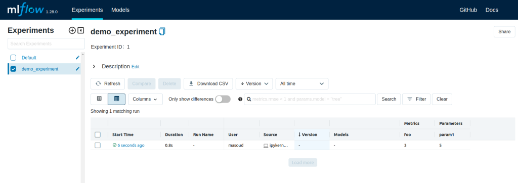
Open the tracking UI by clicking the HTTP link returned: http://127.0.0.1:5000. You can see list of runs for demo_experiment.

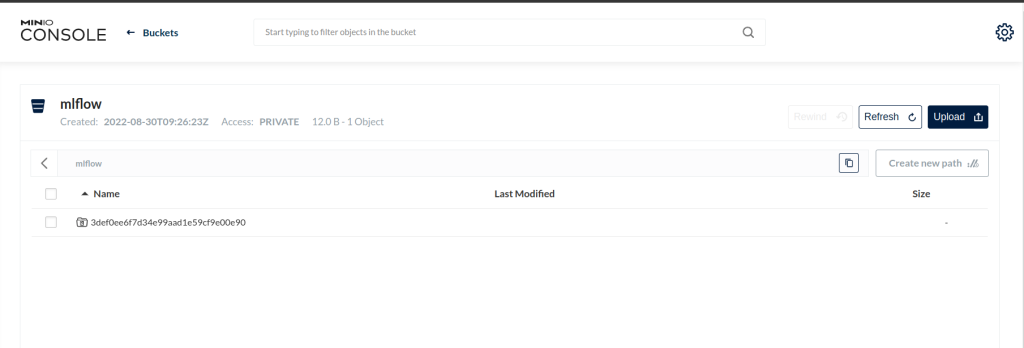
By checking on MinIO console, you can also see that an artifact directory for this run has been created on the mlflow bucket.

MLflow Models

In this example, MLflow Tracking is used to keep track of different hyperparameters, performance metrics, and artifacts of a linear regression model. MLflow Models is used to store the pickled trained model instance, a file describing the environment the model instance was created in, and a descriptor file that lists several “flavors” the model can be used in. MLflow Projects is used to package the training code. And lastly, MLflow Models is used to deploy the model to a simple HTTP server.

This tutorial uses a dataset to predict the quality of the wine based on quantitative features like the wine’s “fixed acidity”, “pH”, “residual sugar”, and so on. The dataset is from UCI’s machine learning repository.

Training the Model

First, train a linear regression model that takes two hyperparameters: alpha and l1_ratio.

This example uses the familiar pandas, numpy, and sklearn APIs to create a simple machine learning model. The MLflow tracking APIs log information about each training run like hyperparameters (alpha and l1_ratio) used to train the model, and metrics (root mean square error, mean absolute error, and r2) used to evaluate the model. The example also serializes the model in a format that MLflow knows how to deploy.

Each time you run the example, MLflow logs information about your experiment runs in the Postgres and Minio.

You can run the example through the train.py script using the following command.

export MLFLOW_TRACKING_URI=postgresql+psycopg2://postgres:postgres@localhost/mlflow_db
export MLFLOW_S3_ENDPOINT_URL=http://127.0.0.1:9000
export AWS_ACCESS_KEY_ID=masoud
export AWS_SECRET_ACCESS_KEY=Strong#Pass#2022
python train.py <alpha> <l1_ratio>

Or you can also use the notebook code below that does the same thing.

def eval_metrics(actual, pred):
    rmse = np.sqrt(mean_squared_error(actual, pred))
    mae = mean_absolute_error(actual, pred)
    r2 = r2_score(actual, pred)
    return rmse, mae, r2

def train(in_alpha, in_l1_ratio):
    np.random.seed(40)

    # Read the wine-quality csv file from the URL
    csv_url = "http://archive.ics.uci.edu/ml/machine-learning-databases/wine-quality/winequality-red.csv"
    data = pd.read_csv(csv_url, sep=";")

    # Split the data into training and test sets. (0.75, 0.25) split.
    train, test = train_test_split(data)

    # The predicted column is "quality" which is a scalar from [3, 9]
    train_x = train.drop(["quality"], axis=1)
    test_x = test.drop(["quality"], axis=1)
    train_y = train[["quality"]]
    test_y = test[["quality"]]

    # Set default values if no alpha is provided
    if float(in_alpha) is None:
        alpha = 0.5
    else:
        alpha = float(in_alpha)

    # Set default values if no l1_ratio is provided
    if float(in_l1_ratio) is None:
        l1_ratio = 0.5
    else:
        l1_ratio = float(in_l1_ratio)

    # Useful for multiple runs
    with mlflow.start_run():
        # Execute ElasticNet
        lr = ElasticNet(alpha=alpha, l1_ratio=l1_ratio, random_state=42)
        lr.fit(train_x, train_y)

        # Evaluate Metrics
        predicted_qualities = lr.predict(test_x)
        (rmse, mae, r2) = eval_metrics(test_y, predicted_qualities)

        # Print out metrics
        print("Elasticnet model (alpha=%f, l1_ratio=%f):" % (alpha, l1_ratio))
        print("  RMSE: %s" % rmse)
        print("  MAE: %s" % mae)
        print("  R2: %s" % r2)

        # Log parameter, metrics, and model to MLflow
        mlflow.log_param("alpha", alpha)
        mlflow.log_param("l1_ratio", l1_ratio)
        mlflow.log_metric("rmse", rmse)
        mlflow.log_metric("r2", r2)
        mlflow.log_metric("mae", mae)
        mlflow.sklearn.log_model(lr, "model")

# Run the above training code with different hyperparameters (9 runs)
alphas = [0.25, 0.5, 0.75]
l1_ratios = [0.25, 0.5, 0.75]
for alpha in alphas:
    for l1_ratio in l1_ratios:
        train(alpha, l1_ratio)

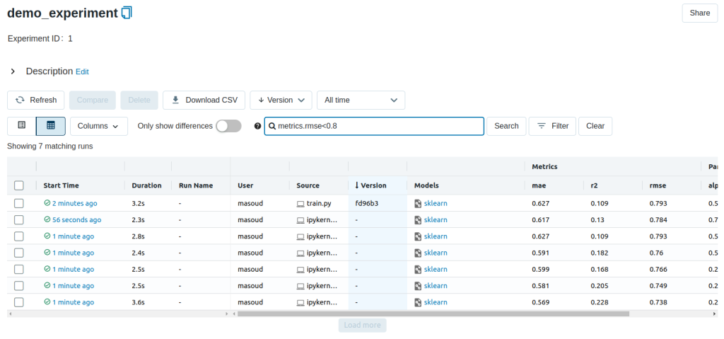
You can use the search feature to quickly filter out many models. For example, the query (metrics.rmse < 0.8) returns all the models with root mean square error less than 0.8. For more complex manipulations, you can download this table as a CSV and use your favorite data munging software to analyze it.

Loading a saved model

After a model has been saved using MLflow Models within MLflow Tracking, you can easily load the model in a variety of flavors (python_function, sklearn, etc.). We need to choose a model from the mlflow bucket in MinIO.

model_path = 's3://mlflow/<run_id>/artifacts/model'
mlflow.<model_flavor>.load_model(modelpath)

import pandas as pd
import numpy as np
import mlflow.sklearn
from sklearn.metrics import mean_squared_error, mean_absolute_error, r2_score
from sklearn.model_selection import train_test_split


def eval_metrics(actual, pred):
    rmse = np.sqrt(mean_squared_error(actual, pred))
    mae = mean_absolute_error(actual, pred)
    r2 = r2_score(actual, pred)
    return rmse, mae, r2


np.random.seed(40)

# Read the wine-quality csv file from the URL
csv_url = "http://archive.ics.uci.edu/ml/machine-learning-databases/wine-quality/winequality-red.csv"
try:
    data = pd.read_csv(csv_url, sep=";")
except Exception as e:
    logger.exception(
        "Unable to download training & test CSV, check your internet connection. Error: %s",
        e,
    )
# Split the data into training and test sets. (0.75, 0.25) split.
train, test = train_test_split(data)
# The predicted column is "quality" which is a scalar from [3, 9]
train_x = train.drop(["quality"], axis=1)
test_x = test.drop(["quality"], axis=1)
train_y = train[["quality"]]
test_y = test[["quality"]]

# Loading the model
loaded_model = mlflow.sklearn.load_model(model_path)

# Evaluate Metrics
predicted_qualities = loaded_model.predict(test_x)
(rmse, mae, r2) = eval_metrics(test_y, predicted_qualities)

# Print out metrics
print("  RMSE: %s" % rmse)
print("  MAE: %s" % mae)
print("  R2: %s" % r2)

Packaging the training code in a conda environment with MLflow projects

Now that you have your training code, you can package it so that other data scientists can easily reuse the model, or so that you can run the training remotely. You do this by using MLflow Projects to specify the dependencies and entry points to your code. The MLproject file specifies that the project has the dependencies located in a conda environment called conda.yaml and has one entry point that takes two parameters: alpha and l1_ratio.

# sklearn_elasticnet_wine/MLproject
name: tutorial

conda_env: conda.yaml

entry_points:
  main:
    parameters:
      alpha: float
      l1_ratio: {type: float, default: 0.1}
    command: "python train.py {alpha} {l1_ratio}"

To run this project use mlflow run on the folder containing the MLproject file. To designate the correct experiment, use the –experiment-name argument. We must set our environment variables in the terminal before running the command.

export MLFLOW_TRACKING_URI=postgresql+psycopg2://postgres:postgres@localhost/mlflow_db
export MLFLOW_S3_ENDPOINT_URL=http://127.0.0.1:9000
export AWS_ACCESS_KEY_ID=masoud
export AWS_SECRET_ACCESS_KEY=Strong#Pass#2022
mlflow run . -P alpha=1.0 -P l1_ratio=1.0 --experiment-name demo_experiment

If a repository has an MLproject file you can also run a project directly from GitHub. This tutorial lives in the https://github.com/iamirmasoud/mlflow_postgres_minio repository which you can run with the following command. The symbol “#” can be used to move into a subdirectory of the repo. The –version argument can be used to run code from a different branch. To designate the correct experiment use the –experiment-name argument. We must set our environment variables in the terminal before running the command.

export MLFLOW_TRACKING_URI=postgresql+psycopg2://postgres:postgres@localhost/mlflow_db
export MLFLOW_S3_ENDPOINT_URL=http://127.0.0.1:9000
export AWS_ACCESS_KEY_ID=masoud
export AWS_SECRET_ACCESS_KEY=Strong#Pass#2022
mlflow run https://github.com/iamirmasoud/mlflow_postgres_minio -P alpha=1.0 -P l1_ratio=0.8 --experiment-name demo_experiment

After running this command, MLflow runs your training code in a new conda environment with the dependencies specified in conda.yaml. You can add –no-conda option to mlflow run command to use the current environment instead of creating a new conda environment for this run.

Serving the Model

Now that you have packaged your model using the MLproject convention and have identified the best model, it is time to deploy the model using MLflow Models. An MLflow Model is a standard format for packaging machine learning models that can be used in a variety of downstream tools – for example, real-time serving through a REST API or batch inference on Apache Spark.

In the example training code, after training the linear regression model, a function in MLflow saved the model as an artifact within the run.

mlflow.sklearn.log_model(lr, "model")

def train_with_model_registry(in_alpha, in_l1_ratio):
    np.random.seed(40)

    # Read the wine-quality csv file from the URL
    csv_url = "http://archive.ics.uci.edu/ml/machine-learning-databases/wine-quality/winequality-red.csv"
    data = pd.read_csv(csv_url, sep=";")

    # Split the data into training and test sets. (0.75, 0.25) split.
    train, test = train_test_split(data)

    # The predicted column is "quality" which is a scalar from [3, 9]
    train_x = train.drop(["quality"], axis=1)
    test_x = test.drop(["quality"], axis=1)
    train_y = train[["quality"]]
    test_y = test[["quality"]]

    # Set default values if no alpha is provided
    if float(in_alpha) is None:
        alpha = 0.5
    else:
        alpha = float(in_alpha)

    # Set default values if no l1_ratio is provided
    if float(in_l1_ratio) is None:
        l1_ratio = 0.5
    else:
        l1_ratio = float(in_l1_ratio)

    # Useful for multiple runs
    with mlflow.start_run():
        # Execute ElasticNet
        lr = ElasticNet(alpha=alpha, l1_ratio=l1_ratio, random_state=42)
        lr.fit(train_x, train_y)

        # Evaluate Metrics
        predicted_qualities = lr.predict(test_x)
        (rmse, mae, r2) = eval_metrics(test_y, predicted_qualities)

        # Print out metrics
        print("Elasticnet model (alpha=%f, l1_ratio=%f):" % (alpha, l1_ratio))
        print("  RMSE: %s" % rmse)
        print("  MAE: %s" % mae)
        print("  R2: %s" % r2)

        # Log parameter, metrics, and model to MLflow
        mlflow.log_param("alpha", alpha)
        mlflow.log_param("l1_ratio", l1_ratio)
        mlflow.log_metric("rmse", rmse)
        mlflow.log_metric("r2", r2)
        mlflow.log_metric("mae", mae)
        mlflow.sklearn.log_model(lr, "model")
        mlflow.sklearn.log_model(
        sk_model=lr,
        artifact_path = "model",
        registered_model_name="ElasticnetWineModel"
    )

train_with_model_registry(0.75, 0.75)

To view this artifact, you can use the UI again. When you click a date in the list of experiment runs you’ll see this page.

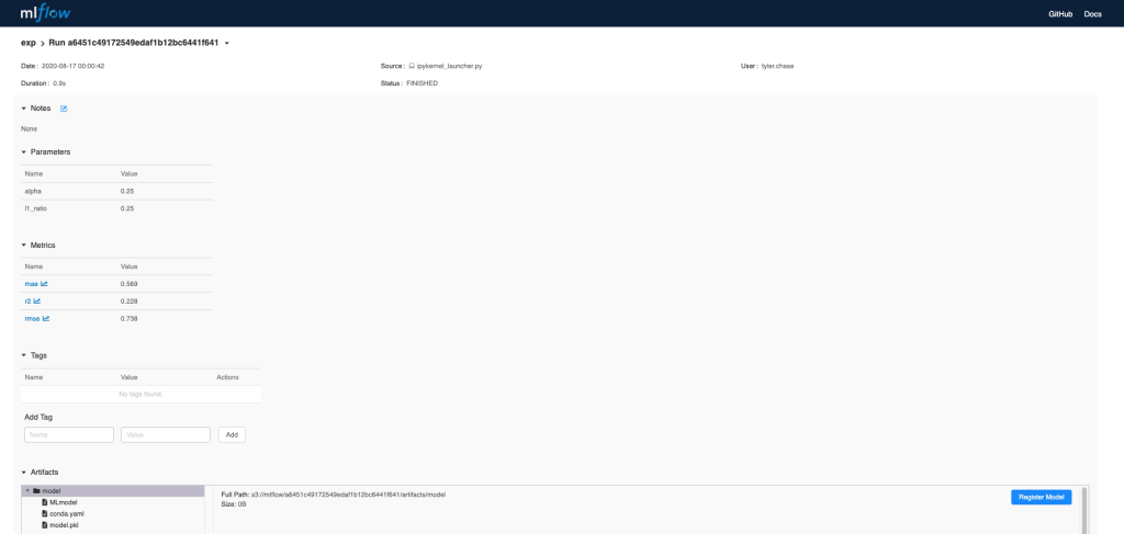
At the bottom, you can see that the call to mlflow.sklearn.log_model produced three files in s3://mlflow/<run_id>/artifacts/model. The first file, MLmodel, is a metadata file that tells MLflow how to load the model. The second file is a conda.yaml that contains the model dependencies from the conda environment. The third file, model.pkl, is a serialized version of the linear regression model that you trained.

In this example, you can use this MLmodel format with MLflow to deploy a local REST server that can serve predictions.

We must set our environment variables in the terminal before running the command. To deploy the server, run the following commands:

export MLFLOW_TRACKING_URI=postgresql+psycopg2://postgres:postgres@localhost/mlflow_db
export MLFLOW_S3_ENDPOINT_URL=http://127.0.0.1:9000
export AWS_ACCESS_KEY_ID=masoud
export AWS_SECRET_ACCESS_KEY=Strong#Pass#2022
mlflow models serve -m s3://mlflow/<run_id>/artifacts/model -p 1234

Note: The version of Python used to create the model must be the same as the one running mlflow models serve. If this is not the case, you may see the error:

UnicodeDecodeError: 'ascii' codec can't decode byte 0x9f in position 1: ordinal not in range(128) or raise ValueError, "unsupported pickle protocol: %d"

Once you have deployed the server, you can pass it some sample data and see the predictions. The following example uses curl to send a JSON-serialized pandas DataFrame with the split orientation to the model server. For more information about the input data formats accepted by the model server, see the MLflow deployment tools documentation.

curl -X POST -H "Content-Type:application/json; format=pandas-split" --data '{"columns":["alcohol", "chlorides", "citric acid", "density", "fixed acidity", "free sulfur dioxide", "pH", "residual sugar", "sulphates", "total sulfur dioxide", "volatile acidity"],"data":[[12.8, 0.029, 0.48, 0.98, 6.2, 29, 3.33, 1.2, 0.39, 75, 0.66]]}' http://127.0.0.1:1234/invocations

The server should respond with output similar to:

[3.7783608837127516]

Reference:

https://medium.com/noodle-labs-the-future-of-ai/introduction-to-mlflow-for-mlops-part-3-database-tracking-minio-artifact-storage-and-registry-9fef196aaf42