Steps to Deploy Django with Postgres, Nginx, and Gunicorn on Ubuntu 18.04
2021-11-04
Walk-forward optimization for algorithmic trading strategies on cloud architecture
2021-12-26Multivariate Gaussian distribution is a fundamental concept in statistics and machine learning that finds applications in various fields, including data analysis, image processing, and natural language processing. It is a probability distribution that describes the probability of multiple random variables being correlated with each other. The process of generating random samples from a multivariate Gaussian distribution can be challenging, particularly when the dimensionality of the data is high. In this post, we will explore the topic of sampling from a multivariate Gaussian distribution and provide Python code examples to help you understand and implement this concept.
Steps:
A widely used method for drawing (sampling) a random vector  from the N-dimensional multivariate normal distribution with mean vector
  and covariance matrix
  works as follows:
- Find any real matrix
 such that
  . When is positive-definite, the Cholesky decomposition is typically used, and the extended form of this decomposition can always be used (as the covariance matrix may be only positive semi-definite) in both cases a suitable matrix is obtained. An alternative is to use the matrix
  obtained from a spectral decomposition
  of . The former approach is more computationally straightforward but the matrices change for different orderings of the elements of the random vector, while the latter approach gives matrices that are related by simple re-orderings. In theory, both approaches give equally good ways of determining a suitable matrix , but there are differences in computation time.
 - Let
 be a vector whose components are N independent standard normal variates (which can be generated, for example, by using the Box–Muller transform).
 - Let be
 . This has the desired distribution due to the affine transformation property.
Python Implementation:
1) Implementing From scratch
# Define the desired distribution to sample from:
d = 2 # Number of dimensions
mean = np.matrix([[0.], [1.]])
covariance = np.matrix([
[1, 0.8],
[0.8, 1]
])
# Compute the Decomposition:
A = np.linalg.cholesky(covariance)
# Sample X from standard normal
n = 50 # Samples to draw
Z = np.random.normal(size=(d, n))
# Apply the transformation
X = A.dot(Z) + mean
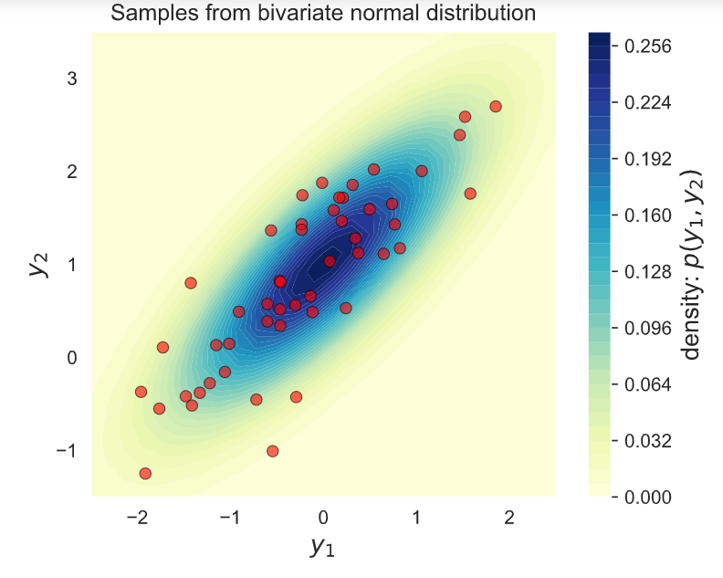
# Plot the samples and the distribution
fig, ax = plt.subplots(figsize=(6, 4.5))
# Plot bivariate distribution
x1, x2, p = generate_surface(mean, covariance, d)
con = ax.contourf(x1, x2, p, 33, cmap=cm.YlGnBu)
# Plot samples
ax.plot(Y[0,:], Y[1,:], 'ro', alpha=.6,
markeredgecolor='k', markeredgewidth=0.5)
ax.set_xlabel('y1', fontsize=13)
ax.set_ylabel('y2', fontsize=13)
ax.axis([-2.5, 2.5, -1.5, 3.5])
ax.set_aspect('equal')
ax.set_title('Samples from bivariate normal distribution')
cbar = plt.colorbar(con)
cbar.ax.set_ylabel('density: p(y1, y2)', fontsize=13)
plt.show()
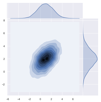
2) Using Numpy Sampler
Numpy has a built-in multivariate normal sampling function:
z = np.random.multivariate_normal(mean=mean, cov=covariance, size=n)
y = np.transpose(z)
# Plot density function.
sns.jointplot(x=y[0], y=y[1], kind="kde", space=0);