Machine Learning Interview: Training Neural Networks

In this post, I will provide the answers to the questions for the online ML interview book.

For more tips on training neural networks, check out:

• A Recipe for Training Neural Networks (Karpathy 2019)
• NLP’s Clever Hans Moment has Arrived (Heinzerling 2019): an excellent writeup on trying to understand what exactly your neural network learns, and techniques to ensure that your model works correctly with textual data.
• An overview of gradient descent optimization algorithms (Ruder 2016)

1) When building a neural network, should you overfit or underfit it first?

Overfit one batch. Overfit a single batch of only a few examples (e.g. as little as two). To do so we increase the capacity of our model (e.g. add layers or filters) and verify that we can reach the lowest achievable loss (e.g. zero). We also like to visualize in the same plot both the label and the prediction and ensure that they end up aligning perfectly once we reach the minimum loss. If they do not, there is a bug somewhere and we cannot continue to the next stage.

So, After getting your model to run, the next thing you need to do is to overfit a single batch of data. This is a heuristic that can catch an absurd number of bugs. This really means that you want to drive your training error arbitrarily close to 0.
There are a few things that can happen when you try to overfit a single batch and it fails:
• Error goes up: Commonly, this is due to a flip sign somewhere in the loss function/gradient.
• Error explodes: This is usually a numerical issue but can also be caused by a high learning rate.
• Error oscillates: You can lower the learning rate and inspect the data for shuffled labels or incorrect data augmentation.
• Error plateaus: You can increase the learning rate and get rid of regulation. Then you can inspect the loss function and the data pipeline for correctness.

2) Write the vanilla gradient update.

The vanilla gradient update rule, also known as stochastic gradient descent (SGD), for updating the parameters of a neural network is:
θ = θ – α * ∇J(θ)
where:
• θ: the parameters of the neural network
• α: the learning rate, which determines the step size of the update
• J(θ): the cost function, which measures the difference between the predicted output and the actual output
• ∇J(θ): the gradient of the cost function with respect to the parameters θ, which indicates the direction of steepest ascent in the loss surface.
The update rule computes the gradient of the cost function with respect to the parameters and moves the parameters in the direction of steepest descent by a step proportional to the learning rate α. The process is repeated for each mini-batch of data until convergence.

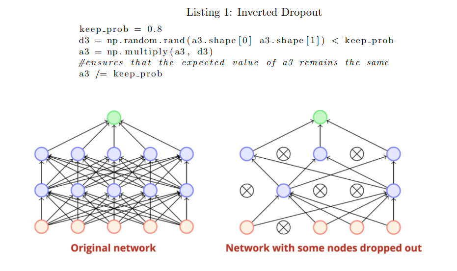
3) Implement vanilla dropout for the forward and backward pass in NumPy.

4) Draw the graphs for sigmoid, tanh, ReLU, and leaky ReLU. Is ReLU differentiable? What to do when it’s not differentiable? Derive derivatives for sigmoid function when is a vector.

Here are the pros and cons of some commonly used activation functions:

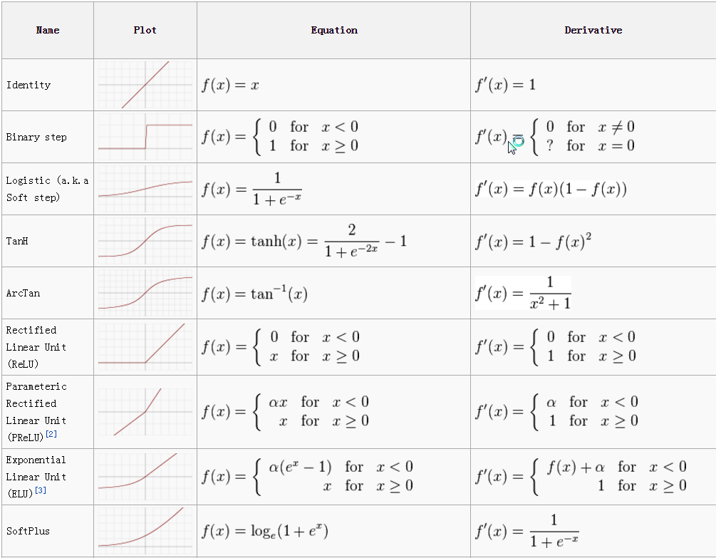
1. Sigmoid:
• Pros: Sigmoid function maps the input to a probability between 0 and 1, which makes it useful in binary classification tasks. It is also differentiable everywhere, which makes it easy to compute gradients for optimization algorithms.
• Cons: The sigmoid function can suffer from vanishing gradients, especially when the input to the function is large or small, which can lead to slower convergence during training. Additionally, the output of the sigmoid function is not zero-centered, which can make it more difficult to train deeper networks.
2. Tanh:
• Pros: The tanh function is zero-centered, which makes it easier to train deeper neural networks. It is also useful in classification tasks where the output label can take on multiple values.
• Cons: Similar to the sigmoid function, the tanh function can suffer from vanishing gradients, especially when the input to the function is large or small.
3. ReLU (Rectified Linear Unit):
• Pros: The ReLU function is simple to compute and is computationally efficient. It has been shown to perform well in many deep learning applications, especially when combined with other techniques such as batch normalization.
• Cons: The ReLU function is not differentiable at x=0, which can lead to issues during backpropagation. Additionally, the ReLU function can suffer from the “dying ReLU” problem, where a neuron can become permanently inactive during training if it receives a large negative input.
4. Leaky ReLU:
• Pros: The Leaky ReLU function addresses the “dying ReLU” problem by allowing some small negative values to pass through, which can help keep the neuron active during training. It has been shown to perform well in many deep learning applications, especially when combined with other techniques such as batch normalization.
• Cons: The Leaky ReLU function is more computationally expensive than the standard ReLU function because it involves an additional parameter. Additionally, the Leaky ReLU function can suffer from the same vanishing gradient problem as the ReLU and tanh functions, especially when the input to the function is large or small.

• ReLU is differentiable for all positive input values (the derivative is 1).
• However, ReLU is not differentiable at exactly x = 0, as the slope changes abruptly.
• To handle non-differentiability, subgradients or “subderivatives” can be used. In the case of ReLU, the subgradient can be defined as:
• f'(x) = 0 if x < 0
• f'(x) = 1 if x > 0
• f'(x) = [0, 1] if x = 0 (this indicates that any value between 0 and 1 is a valid subgradient).

Step 1: Differentiating both sides with respect to x.

Step 2: Apply the reciprocating/chain rule.

Step 3: Modify the equation for a more generalized form.

Vanishing Gradient:

Vanishing gradients refer to the phenomenon where the gradients (derivatives) of the loss function with respect to the weights of earlier layers in a deep neural network become very small during backpropagation. This is particularly problematic for deep neural networks that use activation functions with derivatives that have small values (e.g., sigmoid and tanh functions) since the gradients in such networks can diminish rapidly as they are propagated backwards from the output layer to the input layer.
The problem with vanishing gradients is that it can significantly slow down the training process and sometimes prevent the network from learning effectively. This is because small gradients mean that the weights of earlier layers are updated very slowly, and hence, these layers may not be able to adapt to the data properly. In some cases, the gradients may become so small that they effectively stop the training process altogether, as the weights no longer receive meaningful updates.
However, it’s worth noting that vanishing gradients are less of a problem with activation functions such as ReLU and its variants, which have derivative functions that are not as small as those of sigmoid and tanh functions. Nevertheless, in very deep networks with many layers, vanishing gradients can still occur, particularly if the weights of the network are initialized poorly or if the learning rate is too low.

5) What’s the motivation for skip connection in neural works?

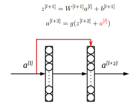
Skip connections, also known as residual connections, were introduced as a solution to the degradation problem in deep neural networks. The degradation problem refers to the observation that as the depth of a neural network increases, its accuracy on the training data saturates and then starts to degrade rapidly, despite the network having enough capacity to fit the data. This is due to the difficulty of optimizing very deep networks, particularly in the presence of vanishing gradients.
Skip connections allow the network to bypass one or more layers, allowing the input to directly connect to the output, or to a later layer in the network. This helps the network to learn identity mappings and to propagate gradients more effectively, which can lead to faster convergence and better accuracy. Skip connections also help to mitigate the vanishing gradient problem by providing a shortcut for gradients to flow through the network.
Overall, the motivation for skip connections is to make it easier to train deeper neural networks that can learn more complex functions, while avoiding the degradation problem and the vanishing gradient problem.

6) How do we know that gradients are exploding? How do we prevent it? Why are RNNs especially susceptible to vanishing and exploding gradients?

How to detect an exploding gradient
There are some key rules that can help identify whether or not the gradient is exploding. These are as follows:
• The model is not performing well on the training data.
• There are large changes in learning loss (unstable learning).
• The loss becomes NaN.
Solution
Some of the suggested solutions to tackle the exploding gradient problem are given below:
• Use batch normalization
• Use less number of layers
• Carefully initialize weights
• Use gradient clipping

Gradients are said to be exploding when their magnitudes become too large during the backpropagation process. This can be observed by monitoring the loss function during training. If the loss function starts to increase rapidly or goes to infinity, it is an indication that gradients may be exploding.
One way to prevent exploding gradients is to use gradient clipping. This involves setting a threshold value and scaling the gradients down if their magnitudes exceed this threshold. This ensures that the gradients remain within a manageable range and do not explode.
Another way to prevent exploding gradients is to use weight initialization techniques. Poorly initialized weights can lead to large gradients, which can result in exploding gradients. Techniques such as Xavier initialization and He initialization can help to ensure that the weights are initialized in a way that prevents the gradients from becoming too large.
Using a smaller learning rate can also help to prevent exploding gradients. A smaller learning rate means that the weights are updated more slowly, which can help to prevent the gradients from becoming too large.
Finally, using batch normalization can also help to prevent exploding gradients. Batch normalization normalizes the activations of the previous layer, which can help to ensure that the gradients are well-behaved and do not become too large.

Recurrent Neural Networks (RNNs) are especially susceptible to vanishing and exploding gradients due to the nature of their recurrent connections and the backpropagation algorithm used for training. The main reasons for this susceptibility are:

1. Repeated Multiplication: RNNs process sequential data by repeatedly applying the same weights and activations over time. This leads to repeated multiplication of the weights during the backpropagation process. If the weights are less than 1 (in the range [0, 1]), the gradients can vanish as they are repeatedly multiplied, resulting in the loss of important information and the network’s inability to learn long-term dependencies. Conversely, if the weights are greater than 1, the gradients can explode and become extremely large, leading to unstable training and difficulty in converging to a solution.
2. Activation Function Choice: The choice of activation function in RNNs can also impact the vanishing and exploding gradient problem. Commonly used activation functions such as sigmoid or tanh have saturation regions where the gradients approach zero for large or small input values. When the network experiences long sequences or deep recurrent connections, the gradients can diminish exponentially or grow exponentially, respectively.
3. Depth of Recurrence: The depth of recurrence in RNNs can amplify the vanishing or exploding gradient issue. As information flows through multiple recurrent layers or time steps, the gradients can accumulate and compound their effect, making the problem more severe. This is particularly problematic when the network needs to capture long-term dependencies or when the sequences are very long.
4. Initialization and Learning Rate: The initialization of weights and the choice of learning rate can also affect the gradient behavior in RNNs. Poorly initialized weights or excessively high learning rates can exacerbate the vanishing or exploding gradient problem.

To mitigate the vanishing and exploding gradient problem in RNNs, several techniques have been developed, including:

• Weight Initialization: Careful initialization of weights, such as using techniques like Xavier or He initialization, can help alleviate the issue by controlling the range of initial weight values.
• Gradient Clipping: Applying gradient clipping, which limits the magnitude of gradients during the training process, can prevent exploding gradients and stabilize training.
• Non-saturating Activation Functions: Using activation functions like ReLU or variants (e.g., Leaky ReLU) can mitigate the vanishing gradient problem as they do not have saturation regions.
• Gate Mechanisms: Architectures like Long Short-Term Memory (LSTM) and Gated Recurrent Unit (GRU) were specifically designed to address the vanishing gradient problem in RNNs. They incorporate gating mechanisms that regulate the flow of information and gradients, allowing for better long-term dependencies.
• Truncated Backpropagation Through Time (BPTT): Instead of backpropagating through the entire sequence, BPTT truncates the sequence into smaller chunks, reducing the propagation of gradients over long distances and mitigating the vanishing/exploding gradients.

These techniques help mitigate the challenges associated with vanishing and exploding gradients in RNNs, enabling more stable and effective training of recurrent neural networks.

7) Weight normalization separates a weight vector’s norm from its gradient. How would it help with training?

Weight normalization is a technique used in neural networks to separate the weight vector’s norm from its gradient. This technique allows the optimizer to adjust the weight vector’s direction and magnitude independently, which can help with training in several ways.
One benefit of weight normalization is that it can improve the convergence of optimization algorithms, especially when using larger learning rates. This is because the norm of the weight vector can be more stable during training, which makes it easier to update the weights without causing instability in the model.
Another benefit of weight normalization is that it can help with the vanishing gradient problem. By separating the norm from the gradient, weight normalization can prevent the gradient from becoming too small and therefore allow information to flow through the network more easily during backpropagation.
Finally, weight normalization can also help with generalization. By normalizing the weight vector, weight normalization can reduce the number of redundant dimensions in the weight space, which can help the model generalize better to new data.
Overall, weight normalization can be a useful technique for improving the training of neural networks by separating the weight vector’s norm from its gradient and providing more stable updates during optimization.

https://sh-tsang.medium.com/review-weight-normalization-a-simple-reparameterization-to-accelerate-training-of-deep-neural-c88fb0918c9b

8) When training a large neural network, say a language model with a billion parameters, you evaluate your model on a validation set at the end of every epoch. You realize that your validation loss is often lower than your train loss. What might be happening?

Dropout
Regularization
Distribution Mismatch
https://towardsdatascience.com/what-your-validation-loss-is-lower-than-your-training-loss-this-is-why-5e92e0b1747e

9) What criteria would you use for early stopping?

Early stopping is a technique used to prevent overfitting in machine learning models. It involves monitoring the performance of the model on a validation set during training and stopping the training process when the model’s performance on the validation set starts to degrade. The criteria used for early stopping depend on the specific problem and model being trained. Here are some common criteria for early stopping:
1. Validation loss: The most common criterion is to monitor the validation loss. When the validation loss stops decreasing or starts to increase, the training is stopped. This criterion assumes that the validation loss is a good proxy for the generalization error of the model.
2. Validation accuracy: In classification problems, it is common to monitor the validation accuracy instead of the validation loss. The training is stopped when the validation accuracy stops improving.
3. Validation F1-score: In some classification problems, it may be more appropriate to monitor the F1-score on the validation set instead of the accuracy.
4. Early stopping with patience: Sometimes, the validation loss or accuracy may fluctuate due to noise or other reasons. In such cases, it may be useful to use early stopping with patience, which involves stopping the training only if the validation loss or accuracy has not improved for a certain number of epochs.
The choice of the early stopping criteria depends on the specific problem and the performance metric that is most relevant to the task. In general, the criterion should be chosen such that it reflects the generalization performance of the model and prevents overfitting.
Patience: Early stopping is a form of regularization, and it can be beneficial to allow the model to overfit slightly before stopping. The patience parameter controls how many epochs the validation loss can increase before training is stopped.
Some more elaborate triggers may include:
• No change in metric over a given number of epochs.
• An absolute change in a metric.
• A decrease in performance observed over a given number of epochs.
• Average change in metric over a given number of epochs.
Some delay or “patience” in stopping is almost always a good idea.

10) Gradient descent vs SGD vs mini-batch SGD.

Gradient descent, SGD (Stochastic Gradient Descent), and mini-batch SGD are optimization algorithms used in training neural networks.
Gradient descent is a batch optimization algorithm that updates the model parameters using the gradients of the loss function computed on the entire training set. It involves computing the gradients for the entire training set, which can be computationally expensive for large datasets. Gradient descent may also get stuck in local minima and saddle points.
SGD is a stochastic optimization algorithm that updates the model parameters using the gradients of the loss function computed on a single training example at a time. This approach is faster than batch gradient descent because it requires only one training example at a time, but it introduces a lot of noise in the gradient estimation, which can make convergence to the optimal solution slower.
Mini-batch SGD is a compromise between the two previous approaches. It updates the model parameters using the gradients of the loss function computed on a small subset of the training set (a mini-batch) at a time. This approach reduces the noise in the gradient estimation and speeds up the computation because it can be done in parallel on a GPU.
In practice, mini-batch SGD is the most commonly used optimization algorithm because it combines the advantages of both gradient descent and SGD. However, the choice of the batch size for mini-batch SGD can have an impact on the convergence rate and the generalization performance of the model.

11) It’s a common practice to train deep learning models using epochs: we sample batches from data without replacement. Why would we use epochs instead of just sampling data with replacement?

When training a deep learning model, it is important to expose the model to as much data as possible to learn the underlying patterns and generalize well on new data. However, training a model on a large dataset can be computationally expensive, and it may not be possible to process all the data at once due to hardware limitations. Therefore, data is often processed in batches during training.
One common practice in deep learning is to train the model using epochs, where the entire dataset is processed in iterations. In each epoch, the data is divided into several batches, and the model is trained on each batch before moving on to the next. The batches are sampled without replacement, which means that each sample in the dataset is used exactly once in each epoch.
The reason for using epochs instead of just sampling data with replacement is to ensure that the model is exposed to all the data during training. If data is sampled with replacement, some samples may be selected more frequently than others, leading to overfitting on those samples and poor generalization to new data. By using epochs and sampling without replacement, each sample in the dataset has an equal chance of being included in each batch, ensuring that the model is exposed to all the data and can learn the underlying patterns better.

12) Your model’ weights fluctuate a lot during training. How does that affect your model’s performance? What to do about it?

Fluctuation in model weights during training is not necessarily an indication of poor model performance. In fact, some degree of fluctuation is expected and can be a sign that the model is adjusting its weights in response to the training data.
However, if the fluctuations are extreme or occur in a repetitive pattern, it may indicate that the model is not converging to a stable solution. This can lead to poor model performance and may require adjustments to the model architecture, hyperparameters, or training process.
To address fluctuating weights, several techniques can be used, including:
1. Regularization: Regularization techniques like L1/L2 regularization or dropout can help to prevent overfitting and stabilize the weights.
2. Learning rate schedule: Adjusting the learning rate during training can help to prevent the weights from fluctuating too much. For example, decreasing the learning rate over time can help the model converge more gradually.
3. Batch normalization: Batch normalization can help to stabilize the distribution of activations in each layer, which can in turn help to stabilize the weights.
4. Early stopping: If the model’s weights are fluctuating but the validation loss is not improving, it may be time to stop training early to prevent the model from overfitting and producing poor results.
By using these techniques, the fluctuations in model weights can be controlled, allowing the model to converge to a stable solution and achieve better performance.

13) Draw a graph number of training epochs vs training error for when the learning rate is:
1. too high
2. too low
3. acceptable.
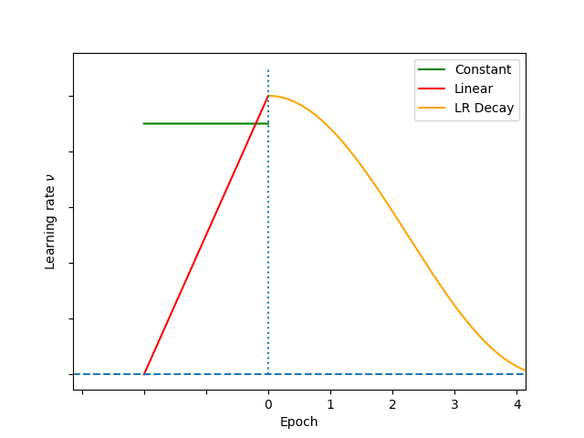
What’s the learning rate warmup? Why do we need it?

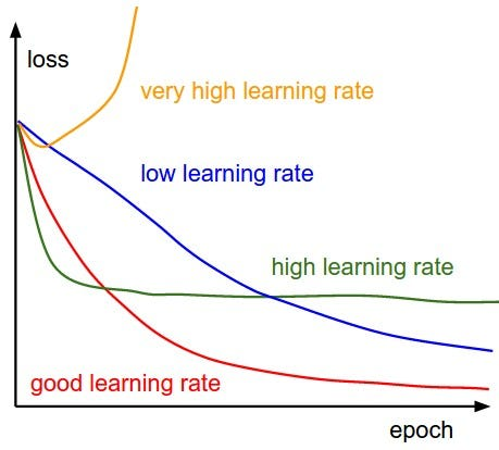
Learning rate warmup is a technique used in training deep learning models where the learning rate is gradually increased from a very small value to the actual learning rate over a certain number of iterations at the beginning of training. The main motivation behind this technique is to prevent the model from diverging or getting stuck in a suboptimal solution during the early stages of training when the model’s weights are randomly initialized and the gradients are large.
When we start training a neural network from scratch, the weights of the network are randomly initialized. At this point, the gradients can be very large, and if we use a large learning rate, the optimization algorithm may overshoot the minima, causing the model to diverge. On the other hand, if we use a very small learning rate, the model will take a long time to converge to the optimal solution. By gradually increasing the learning rate from a small value to the actual learning rate, learning rate warmup allows the optimization algorithm to quickly move in the direction of the minima and avoid divergence or getting stuck in suboptimal solutions.
Learning rate warmup is typically used with optimization algorithms that require a learning rate such as Stochastic Gradient Descent (SGD) or Adam. The length of the warmup period and the rate at which the learning rate is increased can be hyperparameters that need to be tuned for each model and dataset.

For most state-of-the-art architectures, starting to train with a high LR that gradually decreases at each epoch (or iteration) is a commonly adopted adaptive LR strategy. However, this adaptive LR strategy doesn’t always lead to satisfying local optima.

The main reason for using learning rate warmup is to prevent the model from getting stuck in a poor local minimum early in the training process. In the beginning, the model’s weights are randomly initialized, and the gradient values can be quite large, causing the optimizer to overshoot the optimal point and diverge. By gradually increasing the learning rate during the warmup period, we allow the model to explore the parameter space more thoroughly and adjust to the underlying data distribution.
Another benefit of using learning rate warmup is that it can improve the stability and convergence speed of the training process. Gradually increasing the learning rate can help the optimizer to find a smoother trajectory towards the global minimum, avoiding sharp turns and sudden changes in the model’s parameters.

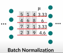
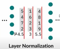
14) Compare batch norm and layer norm.

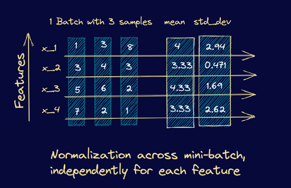
Batch normalization normalizes each feature independently across the mini-batch. Layer normalization normalizes each of the inputs in the batch independently across all features.

Batch normalization and layer normalization are two popular techniques used in deep learning to improve the performance of neural networks. While both techniques aim to address the issue of internal covariate shift, they differ in the way they normalize the inputs.
Batch normalization normalizes the activations of a layer by centering and scaling them based on the mean and variance of the activations in a mini-batch. This technique is typically applied to the outputs of a convolutional or fully connected layer before being passed to the activation function. By doing so, it ensures that the distribution of the activations remains stable during training, which helps in faster convergence and better performance. However, batch normalization is sensitive to batch size and can result in slower training with small batch sizes.

On the other hand, layer normalization normalizes the activations of a layer by centering and scaling them based on the mean and variance of the activations across all channels of a single training sample. This technique is applied to the inputs of each layer, which ensures that the distribution of the activations remains stable regardless of the batch size. Layer normalization is particularly useful in recurrent neural networks, where the input is a sequence of vectors, as it normalizes each vector in the sequence independently.
As batch normalization is dependent on batch size, it’s not effective for small batch sizes. Layer normalization is independent of the batch size, so it can be applied to batches with smaller sizes as well.
Batch normalization requires different processing at training and inference times. As layer normalization is done along the length of input to a specific layer, the same set of operations can be used at both training and inference times.

Normalizing across all features but for each of the inputs to a specific layer removes the dependence on batches. This makes layer normalization well suited for sequence models such as transformers and recurrent neural networks (RNNs) that were popular in the pre-transformer era.
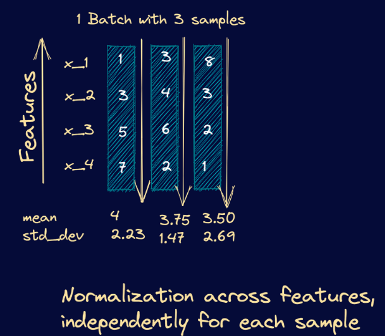
Here’s an example showing the computation of the mean and variance for layer normalization. We consider the example of a mini-batch containing three input samples, each with four features.

From these steps, we see that they’re similar to the steps we had in batch normalization. However, instead of the batch statistics, we use the mean and variance corresponding to specific input to the neurons in a particular layer, say k. This is equivalent to normalizing the output vector from layer k-1.

As an example, let’s consider a mini-batch with 3 input samples, each input vector being four features long. Here’s a simple illustration of how the mean and standard deviation are computed in this case. Once we compute the mean and standard deviation, we can subtract the mean and divide it by the standard deviation.

In summary, batch normalization and layer normalization both address the internal covariate shift problem, but they differ in their normalization methods. Batch normalization is more suitable for feedforward neural networks, while layer normalization is more suitable for recurrent neural networks.

Internal Covariate Shift is the change in the distribution of network activations due to the change in network parameters during training
In neural networks, the output of the first layer feeds into the second layer, the output of the second layer feeds into the third, and so on. When the parameters of a layer change, so does the distribution of inputs to subsequent layers.
These shifts in input distributions can be problematic for neural networks, especially deep neural networks that could have a large number of layers.

It is a phenomenon that occurs in deep learning neural networks when the distribution of input data to each layer changes as the weights of the previous layers are updated during the training process. Specifically, as the parameters of the earlier layers change, the distribution of inputs to the later layers also changes, requiring the later layers to continuously adapt to new distributions of inputs. This results in slower training and lower overall accuracy.
Internal Covariate Shift can be reduced by techniques such as Batch Normalization, which normalizes the inputs to a layer across the batch of data samples to maintain a stable distribution of inputs to each layer throughout the training process. Other techniques such as Weight Normalization and Layer Normalization have also been proposed to address Internal Covariate Shift and improve the efficiency and performance of deep learning neural networks.

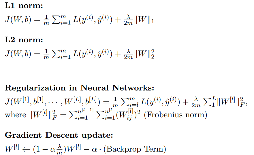
15) Why is squared L2 norm sometimes preferred to L2 norm for regularizing neural networks?

Squared L2 norm, also known as weight decay, is sometimes preferred over L2 norm for regularizing neural networks because it has a more significant effect on larger weights than smaller ones. In neural networks, the weights typically represent the strength of the connections between neurons. Larger weights can lead to overfitting, where the model becomes too complex and performs well on the training data but poorly on new data.
L2 regularization penalizes larger weights by adding a term to the loss function proportional to the L2 norm of the weights. Squaring this term, which is equivalent to applying the squared L2 norm, further amplifies the penalty on larger weights. This can be beneficial because it encourages the model to distribute the weight values more evenly across the neurons, preventing some neurons from dominating others.
Moreover, using the squared L2 norm simplifies the computation of the gradient descent optimization algorithm, which is used to train the neural network. Squaring the term results in a linear equation, which can be efficiently solved using standard linear algebra techniques, while the square root involved in the L2 norm results in a nonlinear equation that requires more complex optimization algorithms.
In summary, using the squared L2 norm for regularization can lead to better generalization performance, encourage the distribution of weight values more evenly, and simplify the computation of the gradient descent algorithm in neural networks.

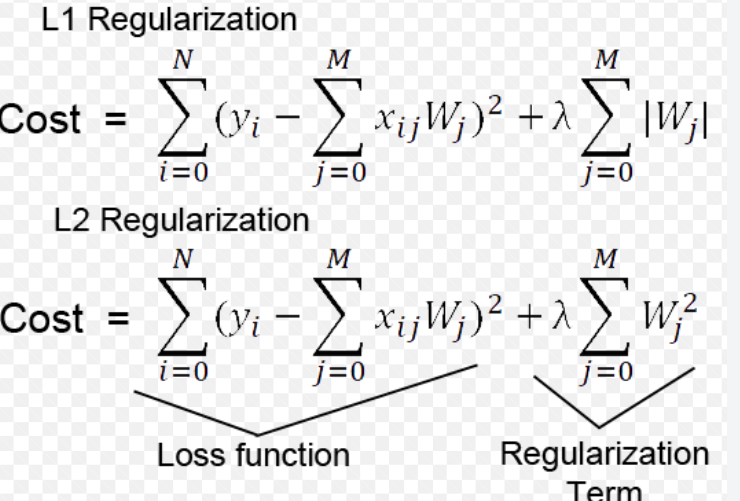
16) Differences between L1 and L2 regularization?

• L1 regularization penalizes the sum of absolute values of the weights, whereas L2 regularization penalizes the sum of squares of the weights. 
• The L1 regularization solution is sparse. The L2 regularization solution is non-sparse.
• L2 regularization doesn’t perform feature selection, since weights are only reduced to values near 0 instead of 0. L1 regularization has built-in feature selection.
• L1 regularization is robust to outliers, L2 regularization is not. 

17) Some models use weight decay: after each gradient update, the weights are multiplied by a factor slightly less than 1. What is this useful for?

Weight decay is a regularization technique used to prevent overfitting in machine learning models, particularly in neural networks. In weight decay, a penalty term is added to the loss function that the model is trying to minimize. The penalty term is proportional to the magnitude of the weights in the model, which encourages the model to learn smaller weights.
Multiplying the weights by a factor slightly less than 1 after each gradient update is a specific implementation of weight decay, known as L2 regularization or ridge regression. This effectively reduces the size of the weights, making the model less likely to overfit to the training data by reducing the model’s capacity.
L2 regularization is often preferred over other forms of regularization because it has a simple interpretation and is computationally efficient. By reducing the size of the weights, it helps to smooth out the decision boundary, leading to a more robust model that is less likely to overfit to noise in the data.
Overall, weight decay is a powerful regularization technique that can help improve the generalization performance of machine learning models, and it is particularly effective in deep neural networks where overfitting is a common problem.

18) It’s a common practice for the learning rate to be reduced throughout the training. What’s the motivation? What might be the exceptions?

The motivation for reducing the learning rate throughout the training is to improve the convergence and stability of the optimization process.

At the beginning of the training, the learning rate is typically set to a relatively high value to allow the model to quickly move towards the minimum of the loss function. However, as the optimization process continues, the model may start to oscillate around the minimum or overshoot it, resulting in slow convergence or even divergence of the optimization process.
By reducing the learning rate over time, the model can take smaller steps towards the minimum of the loss function, allowing it to converge more smoothly and avoid oscillations or overshooting. This approach is often called learning rate annealing or learning rate scheduling.
2. There might be some exceptions where reducing the learning rate throughout the training is not necessary or even harmful. For example:
• If the dataset is small and the model is simple, reducing the learning rate may not provide any significant benefits, as the model may converge quickly even with a constant learning rate.
• If the learning rate is already set to a very low value, reducing it further may slow down the optimization process too much, leading to a longer training time or even getting stuck in a local minimum.
• If the model is trained using adaptive optimization algorithms such as Adam, RMSprop, or Adagrad, the learning rate is often adapted automatically based on the gradient information, and reducing the learning rate manually may interfere with the adaptive mechanism and hurt performance.
In general, the optimal learning rate schedule depends on the specific problem and model architecture, and it is often determined through empirical experimentation.

18) What happens to your model training when you decrease the batch size to 1? What happens when you use the entire training data in a batch? How should we adjust the learning rate as we increase or decrease the batch size?

Reducing the batch size adds more noise to convergence. Smaller samples have more variation from one another, so the convergence rate and direction on the above terrain is more variable. As a result, the model is more likely to find broader local minima. This contrasts with taking a large batch size, or even all the sample data, which results in smooth convergence to a deep, local minimum. Hence, a smaller batch size can provide implicit regularization for your model.

When you decrease the batch size to 1, the model training becomes more stochastic, meaning that the model parameters are updated after each individual sample, rather than after a batch of samples. This can lead to faster convergence in some cases, as the model can quickly adapt to each sample in the training data. However, it can also lead to high variance in the updates, which can make the training more unstable and increase the risk of overfitting.
Furthermore, using a batch size of 1 can significantly slow down the training process, as it may require a large number of iterations to process the entire training dataset. This is because the model has to perform a forward pass and backward pass for each individual sample in the dataset before updating the model parameters. This can make the optimization process computationally expensive, especially for large datasets.

Overall, decreasing the batch size to 1 can be useful in certain situations, such as when working with small datasets or when using online learning, where the model needs to be updated in real-time as new data becomes available. However, it can also be more challenging to optimize and may require careful tuning of the learning rate and other hyperparameters to prevent overfitting and ensure stable training.

When you use the entire training data in a batch, it is called batch gradient descent or full batch gradient descent. In this approach, the model parameters are updated after computing the gradients of the loss function with respect to all samples in the training set.
Using the entire training dataset in a batch can provide more accurate gradient estimates, as it uses all available information in the training data. This can result in faster convergence towards the minimum of the loss function and better generalization performance on the test data.
However, using the entire training dataset in a batch can also be computationally expensive, as it requires computing the gradients for the entire dataset in each iteration. This can make the optimization process more difficult to scale to large datasets and can result in slow training times.

Therefore, while batch gradient descent can be effective for small and moderately sized datasets, it is not always practical for larger datasets. In such cases, stochastic gradient descent (SGD) or its variants, such as mini-batch gradient descent, are often used. These methods update the model parameters based on a small subset of the training data at each iteration, rather than using the entire dataset. This can result in noisier gradient estimates but can also reduce the computational cost and make the optimization process more tractable for large datasets.

Relation Between Learning Rate and Batch Size

As we increase or decrease the batch size, we should adjust the learning rate proportionally to ensure that the optimization process remains stable and effective.

The question arises is there any relationship between learning rate and batch size? Do we need to change the learning rate if we increase or decrease batch size? First of all, if we use any adaptive gradient descent optimizer, such as Adam, Adagrad, or any other, there’s no need to change the learning rate after changing batch size.
Because of that, we’ll consider that we’re talking about the classic mini-batch gradient descent method.
4.1. Theoretical View
There are some works done on this problem. Some authors suggest that when multiplying batch size by k, we should also multiply the learning rate with root(k) to keep the variance in the gradient expectation constant. Also, more commonly, a simple linear scaling rule is used. It means that when the batch size is multiplied by root(k), the learning rate should also be multiplied by root(k), while other hyperparameters stay unchanged.

When adjusting the batch size, it is generally recommended to adjust the learning rate accordingly to maintain training stability and optimize model performance.
The general rule of thumb is that as the batch size increases, the learning rate should also increase. This is because larger batch sizes provide a more stable estimate of the gradient and can support a higher learning rate. Conversely, smaller batch sizes require a lower learning rate to prevent the model from overfitting or oscillating during training.
One common approach to adjusting the learning rate based on batch size is to use a proportional scaling factor. For example, if the original learning rate is lr and the new batch size is bs_new, and the old batch size was bs_old, then the new learning rate lr_new can be calculated as:

https://www.baeldung.com/cs/learning-rate-batch-size

19) Why is Adagrad sometimes favored in problems with sparse gradients?

Adagrad is an algorithm for gradient-based optimization that does just this: It adapts the learning rate to the parameters, performing smaller updates (i.e. low learning rates) for parameters associated with frequently occurring features, and larger updates (i.e. high learning rates) for parameters associated with infrequent features. For this reason, it is well-suited for dealing with sparse data. Dean et al. [10] have found that Adagrad greatly improved the robustness of SGD and used it for training large-scale neural nets at Google, which — among other things — learned to recognize cats in Youtube videos. Moreover, Pennington et al. [11] used Adagrad to train GloVe word embeddings, as infrequent words require much larger updates than frequent ones.

Adagrad is a popular optimization algorithm that is sometimes favored in problems with sparse gradients because it can adaptively adjust the learning rate for each parameter based on its history of gradients.
In problems with sparse gradients, many of the parameters in the model receive updates infrequently or not at all, which can make it challenging to find an appropriate learning rate that is effective for all parameters. Adagrad addresses this challenge by scaling the learning rate for each parameter based on its historical gradients, which allows it to make larger updates for parameters with infrequent updates and smaller updates for frequently updated parameters.
This is achieved by maintaining a separate learning rate for each parameter, which is updated based on the square of the sum of the historical gradients for that parameter. This means that the learning rate is reduced for parameters that have been frequently updated and increased for parameters that have been infrequently updated. By adaptively adjusting the learning rate in this way, Adagrad can effectively handle sparse gradients and converge faster than other optimization algorithms that use a fixed learning rate.
However, it’s worth noting that Adagrad may not always be the best choice for every problem. One potential issue with Adagrad is that it accumulates the squared gradients over time, which can result in a decreasing learning rate and slow convergence. To address this issue, other optimization algorithms such as Adam have been developed, which use a combination of adaptive learning rates and momentum to achieve faster convergence and better performance on a wide range of problems.

20) What can you say about the ability to converge and generalize of Adam vs. SGD? What else can you say about the difference between these two optimizers?

Adam and Stochastic Gradient Descent (SGD) are both optimization algorithms commonly used in deep learning. In general, Adam is known to converge faster than SGD because it utilizes adaptive learning rates and momentum. However, there is no clear consensus on which algorithm is better for generalization.
Adam can sometimes lead to overfitting, which means that the model performs well on the training data but poorly on unseen data. This is because Adam can adapt the learning rate to each individual weight parameter in the network, potentially causing the model to fit the training data too closely.
On the other hand, SGD can sometimes underfit, which means that the model fails to capture the underlying patterns in the data. This is because SGD uses a fixed learning rate and momentum that may not be optimal for all weight parameters in the network.
To address these issues, researchers have proposed variants of Adam and SGD that attempt to balance the trade-off between convergence and generalization. For example, variants of Adam such as AMSGrad and Nadam have been proposed to prevent the algorithm from overshooting the minimum. Additionally, SGD with momentum can be adjusted using techniques such as learning rate schedules and weight decay to improve generalization.
Overall, the choice between Adam and SGD depends on the specific problem and the dataset being used. It is often recommended to try both algorithms and compare their performance on a validation set before deciding which one to use.

21) With model parallelism, you might update your model weights using the gradients from each machine asynchronously or synchronously. What are the pros and cons of asynchronous SGD vs. synchronous SGD?

Asynchronous SGD and synchronous SGD are two different approaches to updating model weights in parallel computing.
In synchronous SGD, all machines or devices that are running the training process are synchronized and update their model weights simultaneously. This means that all machines wait for each other to finish computing gradients before updating their own weights. The advantages of synchronous SGD are that it provides consistent updates across all devices, resulting in better convergence and faster training times. However, it can be limited by the slowest machine in the group, as all machines need to wait for that one to finish before proceeding with the next iteration.
In contrast, asynchronous SGD updates the model weights on each machine independently and asynchronously without waiting for other machines to finish their computations. This allows each machine to work independently at its own pace and can lead to faster training times as the slowest machine does not hold up the others. However, this approach can lead to inconsistencies between the models on different machines, which can make convergence slower and may require more training steps to achieve the same level of accuracy.
Overall, the choice of synchronous or asynchronous SGD depends on the specific training problem, the size of the model and the data, the number of machines, and the communication infrastructure available.

Here are some pros and cons of each approach:
Asynchronous SGD:
• Pros:
◦ Faster training time: Since each machine updates the model weights independently without waiting for others, it can update more frequently and thus achieve faster training time.
◦ Tolerant to machine failures: If one machine fails, the other machines can continue training without being affected.
• Cons:
◦ May converge to a suboptimal solution: Asynchronous updates can introduce noise and inconsistency in the training process, which may lead to suboptimal solutions. Moreover, the different machines may update the model weights in different directions, which can cause oscillations and slow convergence.
◦ Difficult to tune: The learning rate and other hyperparameters may need to be adjusted carefully to prevent divergence or slow convergence.
Synchronous SGD:
• Pros:
◦ Better convergence: Synchronous updates ensure that all machines use the same gradients and update the model weights at the same time, which can lead to better convergence and higher accuracy.
◦ Easier to tune: The hyperparameters can be set globally for all machines, making it easier to tune.
• Cons:
◦ Slower training time: Since all machines need to wait for each other to finish computing gradients and updating the model weights, synchronous updates can be slower than asynchronous updates.
◦ Sensitive to network latency: The training time can be affected by network latency, especially when there are many machines involved.
Overall, the choice between asynchronous SGD and synchronous SGD depends on the specific requirements of the training task and the available resources. Asynchronous SGD may be more suitable for large-scale distributed training with many machines and limited communication bandwidth, while synchronous SGD may be more suitable for smaller-scale distributed training with fewer machines and low network latency.

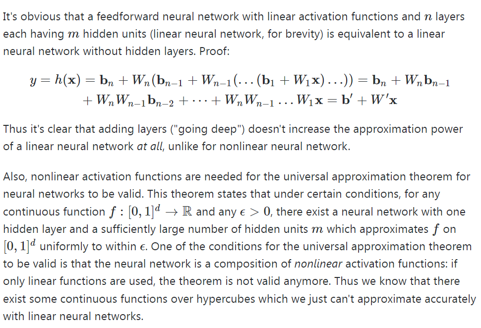
22) Why shouldn’t we have two consecutive linear layers in a neural network?

Using multiple linear layers is basically the same as using a single linear layer. This can be seen through a simple example.
Let’s say you have a one hidden layer neural network, each with two hidden neurons.

Single hidden layer neural network with linear layers
You can then rewrite the output layer as a linear combination of the original input variable if you used a linear hidden layer. If you had more neurons and weights, the equation would be a lot longer with more nesting and more multiplications between successive layer weights. However, the idea remains the same: You can represent the entire network as a single linear layer.
To make the network represent more complex functions, you would need nonlinear activation functions. Let’s start with a popular example, the sigmoid function.

It should be noted that if you are using linear activation functions in multiple consecutive layers, you could just as well have pruned them down to a single layer due to them being linear. (The weights would be changed to more extreme values). Creating a network with multiple layers using linear activation functions would not be able to model more complicated functions than a network with a single layer.

23) Can a neural network with only RELU (non-linearity) act as a linear classifier?

No, a neural network with only ReLU activation function cannot act as a linear classifier. ReLU is a non-linear activation function that introduces non-linearity to the neural network, allowing it to model complex non-linear relationships between inputs and outputs. A linear classifier, on the other hand, is a model that separates data points into different classes using a linear decision boundary.
Without any non-linear activation function, a neural network with only linear layers (also called fully-connected layers or dense layers) can only learn linear relationships between inputs and outputs, and hence it can act as a linear classifier. However, by adding non-linear activation functions like ReLU, the neural network can learn non-linear relationships between inputs and outputs, allowing it to solve more complex tasks beyond linear classification.

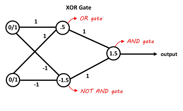
24) Design the smallest neural network that can function as an XOR gate.

25) Why don’t we just initialize all weights in a neural network to zero?

Initializing all weights in a neural network to zero is not a good idea because it leads to the “symmetry problem”. If all weights are the same, then all neurons in the same layer will output the same values, and therefore they will have the same gradient. This means that all weights will be updated in the same way during backpropagation, and the neural network will not be able to learn different features from the input data. In other words, the neural network will not be able to break the symmetry and will not be able to model complex functions.
Instead, we typically initialize the weights randomly using a Gaussian distribution or a uniform distribution. This helps to break the symmetry and allows the neural network to learn different features from the input data. By using random initialization, we also prevent all neurons from having the same gradient during backpropagation, which helps the network to converge faster and achieve better performance.

https://towardsdatascience.com/neural-network-breaking-the-symmetry-e04f963395dd

26) What are some sources of randomness in a neural network? Sometimes stochasticity is desirable when training neural networks. Why is that?

There are several sources of randomness in a neural network:
1. Weight initialization: The initial values of the weights in a neural network are usually chosen randomly. Common methods include Gaussian, uniform, and Xavier initialization, which introduce randomness in the model.
2. Randomness in regularization techniques like Dropouts: Dropout is a regularization technique that randomly drops out some of the neurons during training. This introduces randomness into the model and helps prevent overfitting.
3. Mini-batch sampling: During training, the data is often split into mini-batches. The order of the data in each mini-batch is randomized, and the mini-batches are presented to the model in a random order. This introduces randomness into the optimization process.
4. Stochastic Gradient Descent (SGD): SGD is a popular optimization algorithm used to train neural networks. It randomly selects a subset of the training data (a mini-batch) and computes the gradients based on that subset. This introduces randomness into the optimization process.
5. Data augmentation: Data augmentation techniques such as random cropping, flipping, and rotation are often used to increase the size of the training set. These techniques introduce randomness into the data and can help prevent overfitting.
All of these sources of randomness can help improve the performance of a neural network by preventing overfitting and allowing the model to explore a wider range of solutions.

Stochasticity, or randomness, can be desirable in neural network training for a few reasons:
1. Avoiding local minima: Randomness in the initialization of weights or in the order of training examples presented to the network can help avoid getting stuck in the local minima of the loss function. By exploring different areas of the parameter space, the network has a better chance of finding the global minimum.
2. Regularization: Randomness can be used as a form of regularization to prevent overfitting. For example, dropout is a technique where random neurons are dropped during training, forcing the network to learn redundant representations and increasing its robustness to noise.
3. Exploration: Stochasticity can also be used to explore different parts of the data distribution. By adding noise to the input or the hidden representations, the network can learn to be more robust to variations in the input.
Overall, introducing randomness can help neural networks learn more robust representations, avoid overfitting, and explore different areas of the parameter space.

28) What’s a dead neuron? How do we detect them in our neural network? How to prevent them?

1. A dead neuron is a neuron in a neural network that never activates during the training or inference process, meaning its output is always zero, regardless of the input.
2. Dead neurons can be detected by monitoring the activations of neurons during training or inference. If the output of a neuron is always zero, it is likely a dead neuron.
3. Dead neurons can be prevented by using proper weight initialization methods, such as Xavier or He initialization, which help to avoid saturation of the activation function. Another way to prevent dead neurons is to use activation functions that are less likely to saturate, such as the Leaky ReLU or ELU activation functions. Additionally, using dropout or other regularization techniques can also help prevent dead neurons by forcing the network to learn redundant representations.

https://towardsdatascience.com/neural-network-the-dead-neuron-eaa92e575748

Dying ReLU:

The dying ReLU problem occurs when several neurons only output a value of zero. This happens primarily when the input is negative. This offers an advantage of network sparsity to ReLU, but it creates a major problem when most of the inputs to the neurons are negative. It basically leads to a worst-case scenario when the entire network dies and only a constant function remains.

When most of the neurons output zero, the gradient fails to flow and the weights stop getting updated. Thus, the network stops learning. As the slope of ReLU activation function is zero in the negative input range, once it becomes dead, it is impossible to recover the network to learn.

This dying ReLU problem does not occur quite often because optimizers feed a variety of inputs to the network where in, not all the inputs are in the negative range. As long as the inputs have some positive values, some neurons are active and keep learning as the gradients keeps flowing through the network.

Causes of the Dying ReLU Problem: 

1. High Learning Rate – Let us have a look at the weight updating equation first:

The input to activation function is: (W*x) + b. If the learning rate, alpha value is quite high, it leads to a high probability of the new weights being negative as quite large negative value gets subtracted from our old weights. This further leads to negative inputs to the ReLU function and ultimately causes dying ReLU problem!

2. Higher Negative Bias – While we have mostly taked about negative inputs and higher learning rate, we must not forget that the bias value also gets fed as input when added to the products of inputs and weights. This larger negative bias value might also lead to negative inputs to ReLU function and thus cause dying ReLU problem.

Ways to Solve Dying ReLU Problem: 

1. Lower Learning Rate – As we have seen previously that higher learning rate leads to negative weights, a lower learning rate can help keep this problem in check and reduce the chance of dying ReLU.
2. Other variations of ReLU – As the zero output in the negative input range is the ultimate cause of dying ReLU, we might be better off using other variations of ReLU which adjust the behaviour of the activate function in this range. 

Leaky ReLU is a commonly sought after activation function, which adjusts this flat portion and adds a little slope to it to handle the zero output problem. 

There are other variations of ReLU function, such as parametric ReLU (PReLU), exponential linear unit (ELU), and Gaussian error linear units (GELU) which are also used for the same purpose.

3. Modify the initialization procedure – Symmetric probability distributions, such as He distribution method, are used for the initialization of the neural network. But they are more prone to dying ReLU problem due to the bad local minima.

It has been observed that randomized asymmetric initialization could help prevent dying ReLU problem.

29) Pruning is a popular technique where certain weights of a neural network are set to 0. Why is it desirable? How do you choose what to prune from a neural network?

Pruning is a technique in neural network optimization where certain weights of the network are set to zero, effectively removing connections between neurons. Pruning is desirable for several reasons:

1. Model Efficiency: Pruning reduces the size and complexity of the neural network, leading to improved computational efficiency and reduced memory requirements. Smaller models are faster to train, require less storage, and can be deployed more efficiently on resource-constrained devices.
2. Regularization: Pruning acts as a form of regularization, preventing overfitting by reducing the model’s capacity to memorize noise or irrelevant patterns in the training data. It encourages the network to focus on the most important connections and features, promoting generalization to unseen data.
3. Interpretability: Pruned models are often more interpretable, as the pruned connections can reveal which input features or connections are crucial for the network’s decision-making. Pruning can help identify and understand the most relevant features or connections in the model.

Choosing what to prune from a neural network involves deciding which connections or weights to set to zero. Here are some common approaches for pruning:

1. Magnitude-based Pruning: Weights with the smallest magnitude are pruned. This can be determined by setting a pruning threshold or percentage, such as removing the bottom x% of weights based on their magnitude. The idea is that small magnitude weights contribute less to the network’s output and can be pruned without significant loss of performance.
2. Structured Pruning: Instead of pruning individual weights, entire neurons, channels, or filters can be pruned. This type of pruning exploits the redundancy or unimportance of entire structures within the network. For example, in convolutional neural networks (CNNs), entire convolutional filters can be pruned.
3. Iterative Pruning: Pruning can be performed iteratively over multiple training iterations. After pruning a certain percentage of weights, the model is fine-tuned or retrained to regain performance. This iterative process can be repeated several times, gradually increasing the pruning ratio while maintaining or even improving the model’s accuracy.
4. Data-Driven Pruning: Pruning decisions can be based on additional criteria specific to the data or the network. For example, importance scores based on gradients, sensitivity analysis, or information theoretic measures can guide the pruning process.

It’s worth noting that pruning is often combined with other techniques like weight regularization (e.g., L1 regularization) or knowledge distillation to further enhance the performance and efficiency of pruned models. The choice of pruning method depends on the specific goals, constraints, and characteristics of the neural network and the dataset. Experimentation and fine-tuning of pruning parameters are necessary to strike the right balance between model size, performance, and efficiency.

https://analyticsindiamag.com/a-beginners-guide-to-neural-network-pruning/

https://towardsdatascience.com/pruning-neural-networks-1bb3ab5791f9

30) Under what conditions would it be possible to recover training data from the weight checkpoints?

31) Why do we try to reduce the size of a big trained model through techniques such as knowledge distillation instead of just training a small model from the beginning?

Reducing the size of a big trained model through techniques like knowledge distillation offers several advantages over training a small model from scratch. Firstly, large models often demonstrate superior performance due to their increased capacity for learning complex patterns and representations. By distilling the knowledge from a large model into a smaller one, we can transfer the learned insights, improving the performance of the smaller model without sacrificing accuracy.

Secondly, training a large model from scratch requires substantial computational resources and time-consuming training processes. Knowledge distillation allows us to leverage the knowledge already captured in a pre-trained large model, significantly reducing the training time and computational requirements for the smaller model.

Furthermore, a smaller model is generally more efficient in terms of memory usage and inference speed, making it more practical for deployment in resource-constrained environments such as mobile devices or edge computing platforms. Knowledge distillation enables us to strike a balance between model size and performance, achieving a compact yet effective model.

In summary, knowledge distillation offers the benefits of leveraging the knowledge from a large model, reducing training time and computational requirements, and obtaining a smaller model that is efficient in terms of memory and inference speed. These advantages make it a valuable technique for model compression and deployment in real-world scenarios.