Machine Learning Interview: Objective Functions, Metrics, and Evaluation
2021-06-17
A complete guide on Pandas Grouping, Aggregating, and Transformation
2021-06-26In this article, we’ll be looking at one method for labeling our data and getting it ready for our model. By the end of this article, you should know:
- What labeling is and its importance for machine learning models
- How to use the triple-barrier method to capture events
- What meta-labeling is and why you should use it
Choosing a Learning Approach
There are two general approaches to training machine learning models — supervised and unsupervised learning. The major difference between the two is the existence of a known target output that’s only present in supervised learning. A classic example of supervised learning is linear regression, where given a set of inputs (x) and target outputs (y), we look to create a line of best fit that will predict future target outputs given any arbitrary input.
Within the context of supervised learning, there are two further approaches we can choose from, regression (like the example discussed) or classification. A simple way to think about the difference is to think of regression as the prediction of a continuous quantity while classification is the prediction of a discrete category or label.
An example of classification would be image recognition. In this hilarious scene from HBO’s Silicon Valley, Jian Yang creates an app called “Not Hot Dog” that serves exactly one function — identifying if something is a hot dog or not. For such an app, the underlying model only has two distinct targets or labels to consider for its prediction — “yes it’s a hot dog” or “no it’s not a hot dog”.
For financial stock price prediction, regression seems to make sense here. After all, given that prices are a roughly continuous output, we could simply input all historical data and have it determine a price for some point in the future. Unfortunately, this approach usually fails in practice due to the influence of noise and memory in price data as well as the propensity for over-fitting. Alternatively, we can choose to use classification for our forecasting model. Instead of trying to predict the next price point, we can choose to predict whether intervals of data are pointing us towards a “Buy” or “Sell” classification. In the next section, we’ll discuss how to determine a good labeling strategy.
The Issue with Standard Labelling Strategies
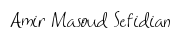
In most modern machine learning research, a form of classification known as the fixed-time horizon method is used. This method involves labeling the returns of our strategy at fixed-time intervals according to fixed thresholds to determine if a label should be “Buy” (if the returns exceed a certain threshold), “Sell” (if the returns dip below a certain threshold), or “Hold” (if the returns are somewhere between the two thresholds).
de Prado notes three primary issues with this approach:
- Time bars (which exhibit poor statistical properties) are used.
- The fixed thresholds make it difficult to accurately label predictions due to the inherent intraday volatility. If we set our thresholds too close together, we will generate many “Buy” and “Sell” signals but most returns will likely be razor-thin. On the other hand, if our thresholds are too far apart, we’ll generate more high-quality signals but miss significant yet predictable trends during low volatility periods (e.g. night trading).
- The thresholds don’t take standard portfolio management principles like profit-taking or stop-loss limits into account. If a position drops 50% in value but then recovers to where it began by the time threshold, this strategy would label the period as a “Hold”, even though any real-world manager would have closed the position. As such, it is important that we take into account the path traveled by the prices instead of exclusively focusing on their final position.
The Triple Barrier Method (TBM)
To overcome the challenges we discussed above, de Prado introduces a labeling technique known as the triple barrier method.
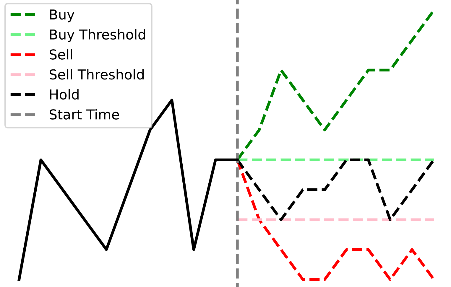
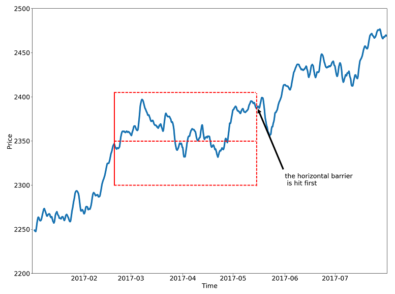
The triple barrier method involves “labeling an observation according to the first barrier touched of out three barriers… two horizontal barriers and one vertical barrier”.
The horizontal barriers can be thought of as profit-taking or stop-loss limits. Rather than setting a fixed threshold, de Prado recommends using a dynamic function that calculates a rolling threshold based on daily volatility. This would allow us to set more optimal thresholds based on recent performance.
The vertical barrier serves as the equivalent of the expiration limit defined by the number of bars elapsed (as opposed to time). This ensures that sampling ranges are roughly equivalent in terms of market activity as opposed to an arbitrary time period.
In short, we have three possible scenarios with two possible outcomes:
- The upper barrier (profit-take) is hit first. Label = “buy” or “1”.
- The lower barrier (stop-loss) is hit first. Label = “sell” or “-1”.
- The vertical barrier (expiration) is hit first. Label = “buy” or “sell” based on the return achieved at expiration.
Implementing the Triple Barrier Method
To view all of the code, please follow along with this Google Colaboratory notebook. To run the code yourself and make changes, make sure to select File -> Save a copy in Drive.
The first part of the code requires us to import processed dollar bars, a technique I describe in this post. If you wish to download a copy of the data I’m using to follow along, you can do so here.
To implement the TBM, we can break down the process into a few steps:
- Use price volatility to determine dynamic thresholds for the upper and lower barriers.
- Determine a signal/trigger for initializing the TBM.
- Add vertical barriers based on trigger times.
- Determine the timestamp of the first touch for each trigger.
1. Determining Daily Volatility
To create our moving thresholds, de Prado recommends setting them based on the prices’ approximate daily movement over the last 100 days with an emphasis on the most recent past (i.e. exponentially weighted moving average).
We’ll begin by using the function, get_daily_vol, to determine a volatility level we want to use as our baseline.
2. Creating a Trigger
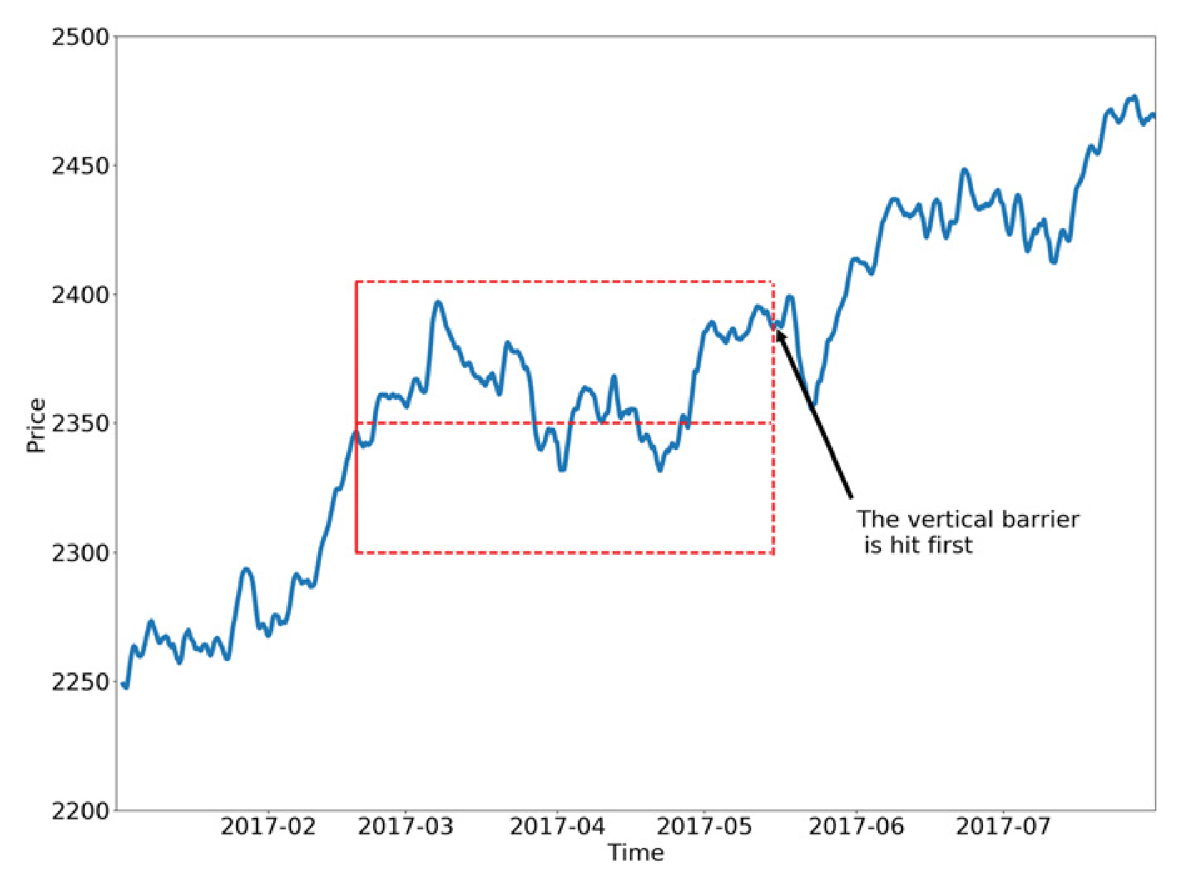
Recall fixed-time horizon labeling, where we simply divide our price series neatly into equally sized sections based on some passage of time (e.g. a day). With TBM, we can no longer use time as our method for determining when each “event”, or series of tracked price changes, begins. Rather, we need to create our own trigger to signal the beginning of each new window.
de Prado recommends using a Symmetric CUSUM Filter as a method for “detecting a shift in the mean value of a measured quantity away from a target value.” (de Prado, 38). The filter is set up to use the daily volatility we derived above to determine the threshold for labeling an event. For example, if our average volatility is 2%, once we exceed a 2% net change since our last event, we would generate a new event and reset our filter.
One advantage of using the CUSUM filter as opposed to traditional technical analysis is that the triggers will not be confused by prices hovering at a threshold level (e.g. RSI of 70). Once each event is triggered, prices must make a certain net delta movement to mark the next event. To attain the position of each event, we can use the function, get_t_events, to help us generate the respective timestamps of each touch.
3. Adding Vertical Barriers
Once we have our list of event timestamps, we can use the function add_vertical_barrier to output a series of all the timestamps when the vertical barrier is reached. We can adjust the argument num_days to the amount of time we want the barrier to stay active.
4. Determining Time of First Touch
The function apply_pt_sl_on_t1 applies the triple barrier labels and outputs a dataframe with the timestamps at which each barrier was touched. We want to use the apply_pt_sl_on_t1within the function get_events to incorporate the results of the previous functions. get_eventsalso allows us the ability to incorporate the side of a bet (decided by a separate primary model) in order to effectively use profit-take and stop-loss limits. That last sentence will make more sense after we describe meta-labeling and move on to the implementation aspect of this article.
Meta-labelling
If we recall the basic purpose of the TBM, the model is designed to produce labels of “Buy”, and “Sell” to guide us into taking long or short positions. However, it is unclear as to how much we should commit to each bet — or whether we should take the bet at all. At this point we have decided on a direction — but not on a bet size.
Meta-labelling is the concept of using a secondary ML model that uses the results of the primary TBM model (which side to bet on) in order to determine whether we should make the bet at all. The primary goal of meta-labeling is to increase our overall success rate in identifying positive trading opportunities. To understand this better, let’s take a look at a simple confusion matrix.
A confusion matrix is a visual representation of the performance of a classification model (like the TBM). In a basic case with a binary classifier (two outputs), you can create a 2×2 table like the one above.
The columns represent the true value of each event — whether it was positive or negative. The rows represent the predicted value by our model. With any model, there will be a number of correct predictions that match the true event (true positives or negatives), as well as predictions that are incorrect (false positives or negatives).
There are two important ratios from this confusion matrix that matter to us with our model — recall and precision.
Recall, or the “true positive rate” is the ratio of true positives / real positives, or how often the model gets a real positive prediction correct. In most cases, as models become more sensitive and better at recall, the rates of false positives also increase, limiting the utility of the model.
Precision is the ratio of true positives / predicted positives. It effectively answers the question: for positive predictions, how often is our model correct?
For a financial model, we want to maximize our recall (correctly capturing all positive trading opportunities) as well as our precision (minimizing our false-positive rates). Because passing up a good opportunity (false negative) is usually less damaging than losing money on a bad opportunity (false positive), we’re less worried about our model’s accuracy with false negatives.
The beauty of incorporating meta-labeling is that we can build an initial model that maximizes recall, even if we have many false positives, and then incorporate a second model that filters out the false positives to enhance our precision score.
Putting It All Together
We’ll be using the following plan to build and test our primary model — then compare it with a meta-labeled model:
- Build a simple bollinger band strategy to identify long and short signals
- Apply the TBM techniques outline above to determine our triple barrier events
- Use forecasts from the primary model to generate meta-labels
- Use a random forest algorithm on the meta-labels to filter the “Buy” and “Sell” decisions and improve the overall precision of the model
This part of the code can be quickly accessed here.
Building our Primary Model
We begin by importing our preprocessed dollar bars. If you’re using the same dataset as me, it should look something like this:
#   Column  Non-Null Count   Dtype
---  ------  --------------   -----
 0   open    200320 non-null  float64
 1   high    200320 non-null  float64
 2   low     200320 non-null  float64
 3   close   200320 non-null  float64
We’ll then use a simple bollinger band model to determine the initial signals for our strategy.
Determining Triple Barrier Events
From here we can implement our triple barrier method to obtain our dataframe of triple_barrier_events — or the timestamps of when each barrier was the first touched.
Generating Meta-labels
We’ll then use a new function get_bins to meta-label each event with a 0 or a 1 based on whether or not the primary model achieved the correct prediction. You can think about this logic like this:
- If our primary model (side) indicated a position and our return at the end of the triple barrier event was positive, we would label that “bin” as a 1 (true positive).
- If our primary model (side) indicated a position and our return at the end of the triple barrier event was negative, we would label that “bin” as a 0 (false positive).
The important concept to understand here is that we have three main categories of classifiers (primary model, triple barrier events, and bin labels) which all output some variation of {-1,0,1} but have distinct purposes. Do not get these three confused! At this point, we can evaluate the performance of our initial model using the bin labels we just generated. Your results should look something like this:
                precision    recall  f1-score   support

           0       0.00      0.00      0.00      7862
           1       0.22      1.00      0.36      2168

    accuracy                           0.22     10030
   macro avg       0.11      0.50      0.18     10030
weighted avg       0.05      0.22      0.08     10030

Confusion Matrix
[[   0 7862]
 [   0 2168]]

Accuracy
0.21615154536390827
As we can see, our initial model achieved an accuracy score of just 22%. Let’s see if we can increase this score.
Applying our Secondary Model
We’ll be using a random forest classifier as our secondary model. We will be using all features of our dataset for training and setting our “bin” labels as the predicted feature. The goal here is to train the model to decide whether to take the bet or pass, a purely binary prediction.
If we look at our performance with the secondary model on the test set:
                precision    recall  f1-score   support

           0       0.82      0.31      0.45      1532
           1       0.26      0.78      0.39       474

    accuracy                           0.42      2006
   macro avg       0.54      0.54      0.42      2006
weighted avg       0.68      0.42      0.43      2006

Confusion Matrix
[[ 469 1063]
 [ 106  368]]

Accuracy
0.4172482552342971
Right away we can see a dramatic increase in our accuracy score from 22% to 42%. This also included an improvement in our precision score from 22% to 26%, meaning we’re getting almost 20% more of our trades correct.
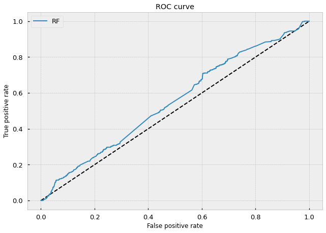
If we take a look at the ROC curve, we can tell by the rise above the middle dotted line that our model has decent predictive power in distinguishing between good trading opportunities (true positives) and poor ones (false negatives).
Labeling Observations
In the financial context, a simple approach for a supervised learning problem is to try to predict the price of an instrument at some fixed horizon in the future. Note that this is a regression task, i.e. we’d attempt to predict a continuous random variable. This is a hard problem to solve because prices are notoriously noisy and serially correlated, and the set of all possible price values is technically infinite. On the other hand, we can approach this as a classification problem — instead of predicting the exact price, we can predict discretized returns.
Most financial literature uses fixed-horizon labeling methods, i.e. the observations are labeled according to returns some fixed number of steps in the future. The labels are discretized by profit and loss thresholds:
This labeling method is a good start, but it has two addressable problems.
- The thresholds are fixed, but volatility isn’t — meaning that sometimes our thresholds are too far apart and sometimes they are too close together. When the volatility is low (e.g. during the night trading session) we will get mostly y=0 labels even though the low returns are predictable and statistically significant.
- The label is path-independent, meaning that it only depends on the return at the horizon and not the intermediate returns. This is a problem because the label doesn’t accurately reflect the reality of trading — every strategy has a stop-loss threshold and a take-profit threshold which can close the position early. If an intermediate return hits the stop-loss threshold, we will realize a loss, and holding the position or profiting from it is unrealistic. Conversely, if an intermediate return hits a take-profit threshold we will close it to lock in the gain, even if the return at the horizon is zero or negative.
Computing Dynamic Thresholds
To address the first problem, we can set dynamic thresholds as a function of rolling volatility. We’re assuming that we already have OHLC bars at this point. I use the dollar bars of BitMex:XBT, the bitcoin perpetual swap contract from the previous post — this code snippet will help you catch up if you are starting from scratch.
Here we will estimate the hourly volatility of returns to compute profit and loss thresholds. Below you’ll find a slightly modified function directly from Lopez De Prado, with comments added for clarity:
def get_vol(prices, span=100, delta=pd.Timedelta(hours=1)):
  # 1. compute returns of the form p[t]/p[t-1] - 1  # 1.1 find the timestamps of p[t-1] values
  df0 = prices.index.searchsorted(prices.index - delta)
  df0 = df0[df0 > 0]  # 1.2 align timestamps of p[t-1] to timestamps of p[t]
  df0 = pd.Series(prices.index[df0-1],
           index=prices.index[prices.shape[0]-df0.shape[0] : ])  # 1.3 get values by timestamps, then compute returns
  df0 = prices.loc[df0.index] / prices.loc[df0.values].values - 1  # 2. estimate rolling standard deviation
  df0 = df0.ewm(span=span).std()
  return df0
Adding Path Dependency: Triple-Barrier Method
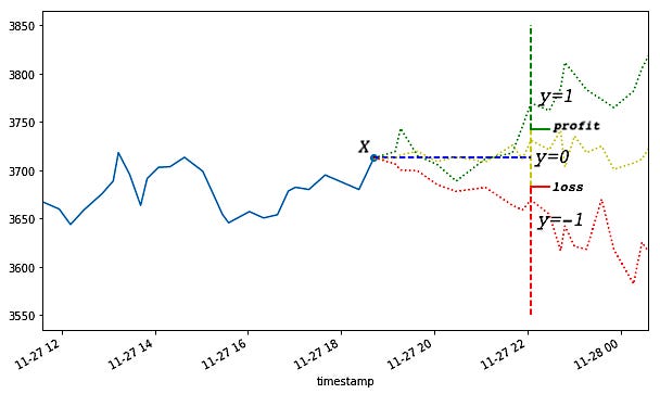
To better incorporate the stop-loss and take-profit scenarios of a hypothetical trading strategy, we will modify the fixed-horizon labeling method so that it reflects which barrier has been touched first — upper, lower, or horizon. Hence the name: the triple-barrier method.
The labeling schema is defined as follows:
y=1: the top barrier is hit first
y=0: the right barrier is hit first
y=-1: the bottom barrier is hit first
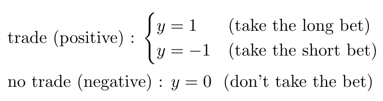
What about the side of the bet?
The schema above works fine for long-only strategies, however, things get more complicated when we allow for both long and short bets. If we are betting short, our profit/loss is inverted relative to the price action — we profit if the price goes down and we lose when the price goes up.
In order to account for this, we can simply represent the side as 1 for long and -1 for short. Thus we can multiply our returns by the side, so whenever we’re betting short the negative returns become positive and vice-versa. Effectively, we flip the y=1 and y=-1 labels if side=-1.
Let’s take a shot at the implementation (based on MLDP’s code).
First, we define the procedure for getting the timestamps of the horizon barriers:
def get_horizons(prices, delta=pd.Timedelta(minutes=15)):
    t1 = prices.index.searchsorted(prices.index + delta)
    t1 = t1[t1 < prices.shape[0]]
    t1 = prices.index[t1]
    t1 = pd.Series(t1, index=prices.index[:t1.shape[0]])
    return t1
Now that we have our horizon barriers, we define a function to set upper and lower barriers based on the volatility estimates computed earlier:
def get_touches(prices, events, factors=[1, 1]):
  '''
  events: pd dataframe with columns
    t1: timestamp of the next horizon
    threshold: unit height of top and bottom barriers
    side: the side of each bet
  factors: multipliers of the threshold to set the height of
           top/bottom barriers
  '''  out = events[['t1']].copy(deep=True)
  if factors[0] > 0: thresh_uppr = factors[0] * events['threshold']
  else: thresh_uppr = pd.Series(index=events.index) # no uppr thresh
  if factors[1] > 0: thresh_lwr = -factors[1] * events['threshold']
  else: thresh_lwr = pd.Series(index=events.index)  # no lwr thresh  for loc, t1 in events['t1'].iteritems():
    df0=prices[loc:t1]                              # path prices
    df0=(df0 / prices[loc] - 1) * events.side[loc]  # path returns
    out.loc[loc, 'stop_loss'] = \
      df0[df0 < thresh_lwr[loc]].index.min()  # earliest stop loss
    out.loc[loc, 'take_profit'] = \
      df0[df0 > thresh_uppr[loc]].index.min() # earliest take profit
  return out
Finally, we define a function to compute the labels:
def get_labels(touches):
  out = touches.copy(deep=True)
  # pandas df.min() ignores NaN values
  first_touch = touches[['stop_loss', 'take_profit']].min(axis=1)
  for loc, t in first_touch.iteritems():
    if pd.isnull(t):
      out.loc[loc, 'label'] = 0
    elif t == touches.loc[loc, 'stop_loss']:
      out.loc[loc, 'label'] = -1
    else:
      out.loc[loc, 'label'] = 1
  return out
Putting it all together:
data_ohlc = pd.read_parquet('data_dollar_ohlc.pq')
data_ohlc = \
  data_ohlc.assign(threshold=get_vol(data_ohlc.close)).dropna()
data_ohlc = data_ohlc.assign(t1=get_horizons(data_ohlc)).dropna()
events = data_ohlc[['t1', 'threshold']]
events = events.assign(side=pd.Series(1., events.index)) # long only
touches = get_touches(data_ohlc.close, events, [1,1])
touches = get_labels(touches)
data_ohlc = data_ohlc.assign(label=touches.label)
Meta-Labeling
On a conceptual level, our goal is to place bets where we expect to win and not to place bets where we don’t expect to win, which reduces to a binary classification problem (where the losing case includes both betting on the wrong direction and not betting at all when we should have). Here’s another way to look at the labels we just generated:
A binary classification problem presents a trade-off between type-I errors (false positives) and type-II errors (false negatives). Increasing the true positive rate usually comes at the cost of increasing the false positive rate.
To characterize this more formally, let us first define:
ŷ ∈ {0, 1, -1} : prediction of the primary model for the observation
r: price return for the observation
Then at prediction time, the confusion matrix of the primary model looks like the one below.
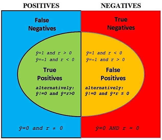
We are not too worried about the false negatives — we might miss a few bets but at least we’re not losing money. We are most concerned about the false positives — this is where we lose money.
To reflect this, our meta-labels y* can be defined according to the diagram:
y*=1:true positive
y*=0:everything but true positive
In effect, the primary model should have high recall — it should identify more of the true positives correctly at the expense of many false positives. The secondary model will then filter out the false positives of the first model.
Meta-Labeling Implementation
First, we create a primary model. Before we do so, an important preprocessing step is to make sure that our training data has balanced labels.
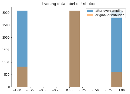
The labels in the original dataset are heavily dominated by 0 values, so if we train on those, we get a degenerate model that predicts 0 every time. We deal with this by applying the synthetic minority over-sampling technique to create a new training dataset where the label counts are roughly equal.
from imblearn.over_sampling import SMOTE
X = data_ohlc[['open', 'close', 'high', 'low', 'vwap']].values
y = np.squeeze(data_ohlc[['label']].values)
X_train, y_train = X[:4500], y[:4500]
X_test, y_test = X[4500:], y[4500:]
sm = SMOTE()
X_train_res, y_train_res = sm.fit_sample(X_train, y_train)
Next, we fit a logistic regression model to our resampled training data. Note that at this point we should not expect our model to do well because we haven’t generated any features, but we should still see an improved F1 score when using meta-labeling over the baseline model.
from sklearn.linear_model import LogisticRegression
clf = LogisticRegression().fit(X_train_res, y_train_res)
y_pred = clf.predict(X_test)
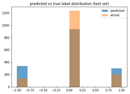
We can see that our model predicts more 1’s and -1’s than there are in our test data. The blue portions of the leftmost and rightmost columns represent the false positives, which we intend to eliminate by meta-labeling and training the secondary model.
Let’s map our triple-barrier predictions into binary positive/negative meta-labels introduced earlier and check the confusion matrix:
def true_binary_label(y_pred, y_test):
    bin_label = np.zeros_like(y_pred)
    for i in range(y_pred.shape[0]):
        if y_pred[i] != 0 and y_pred[i]*y_test[i] > 0:
            bin_label[i] = 1  # true positive
    return bin_labelfrom sklearn.metrics import confusion_matrix
cm= confusion_matrix(true_binary_label(y_pred, y_test), y_pred != 0)
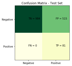
As expected, we see no false negatives and a lot of false positives. We will try to reduce the false positives without adding too many false negatives.
# generate predictions for training set
y_train_pred = clf.predict(X_train)
# add the predictions to features
X_train_meta = np.hstack([y_train_pred[:, None], X_train])
X_test_meta = np.hstack([y_pred[:, None], X_test])
# generate true meta-labels
y_train_meta = true_binary_label(y_train_pred, y_train)
# rebalance classes again
sm = SMOTE()
X_train_meta_res, y_train_meta_res = sm.fit_sample(X_train_meta, y_train_meta)
model_secondary = LogisticRegression().fit(X_train_meta_res, y_train_meta_res)
y_pred_meta = model_secondary.predict(X_test_meta)
# use meta-predictions to filter primary predictions
cm= confusion_matrix(true_binary_label(y_pred, y_test), (y_pred * y_pred_meta) != 0)
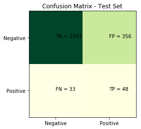
The results in the secondary model show that we introduce a few false negatives, but we eliminate over 30% of false positives from the primary model. While it isn’t always a worthy trade-off, remember the context of trading — we miss out on some trading opportunities (false negatives), but that is a cheap price to pay for cutting down many trades that blow up in our faces (false positives). The classification report confirms our intuition that the efficiency of the classifier improves as measured by the F1 score.
# WITHOUT META-LABELING       label    precision    recall  f1-score   support

           0       1.00      0.66      0.79      1499
           1       0.14      1.00      0.24        81

   micro avg       0.67      0.67      0.67      1580
   macro avg       0.57      0.83      0.52      1580
weighted avg       0.96      0.67      0.76      1580# WITH META-LABELING       label    precision    recall  f1-score   support

           0       0.97      0.76      0.85      1499
           1       0.12      0.59      0.20        81

   micro avg       0.75      0.75      0.75      1580
   macro avg       0.55      0.68      0.53      1580
weighted avg       0.93      0.75      0.82      1580
While neither model is great, remember that we are merely demonstrating a technique for improving classifier efficiency, which can conceivably work well on a larger dataset, better model, and more powerful features.
Meta-Labeling: Quantamental Approach
In general, the interpretation of meta-labeling + secondary model is to predict the confidence level of the primary model. In our example, both the primary and the secondary models were data-driven, but this doesn’t always have to be the case.
In addition to improving F1 scores, meta-labeling has another extremely powerful application — it can add a machine learning layer on top of non-ML models, including econometric forecasts, fundamental analysis, technical signals, and even discretionary strategies. This offers a powerful combination of human intuition/expertise and quantitative edge that is favored by many asset managers for its explainability and robustness.
Next Steps
This example involved a super basic primary model (Bollinger bands) and a bare-bones secondary model (only training on price features). The performance could be improved by either using a better primary model or using more features for the secondary model.
Additionally, many of the parameters I used for triple barrier labeling were default parameters that were not tuned for the asset. You could attempt different values for the daily volatility, the CUSUM filter, the vertical barrier expiration timing, and more.
Conclusion
In today’s article, we looked at implementing a basic model using the triple barrier method and meta-labeling. We learned about using classification for financial machine learning, different ways of labeling data, and the benefits of meta-labeling. Next time, we’ll look at ways of improving our secondary model — such as using fractionally differentiated features to increase the stationarity of our data.
References
https://ai.plainenglish.io/start-using-better-labels-for-financial-machine-learning-6eeac691e660
https://towardsdatascience.com/financial-machine-learning-part-1-labels-7eeed050f32e
https://docs.mizar.ai/mizar/mizarlabs/transformations/labeling-methods
https://quantdare.com/4-simple-ways-to-label-financial-data-for-machine-learning/
A Quantamental Approach Using Labeling for Stock Trading – Lucena Research
https://lucenaresearch.com/2019/03/27/quantamental-approach-to-stock-trading/
Data Rounder – Labeling for Supervised Learning in Finance
https://jjakimoto.github.io/articles/finance_labeling/
A Dynamic Labeling Approach for Financial Assets Forecasting – Lucena Research
https://lucenaresearch.com/2020/02/26/a-dynamic-labeling-approach-for-financial-assets-forecasting-2/
Meta Labeling (A Toy Example) – Hudson & Thames
https://hudsonthames.org/meta-labeling-a-toy-example/
Codes:
https://gist.github.com/davidzhaodz
https://github.com/BlackArbsCEO/Adv_Fin_ML_Exercises/blob/master/src/features/snippets.py
Further Readings:
- Advances in Financial Machine Learning by Marcos Lopez de Prado
- Financial Machine Learning Part 0: Bars by Maks Ivanov
- Financial Machine Learning Part 1: Labels by Maks Ivanov
- Advances in Financial Machine Learning Exercises by BlackArbsCEO
- Machine Learning Financial Laboratory (MlFinLab) by Hudson and Thames
- Does Meta Labeling Add to Signal Efficacy? by Ashutosh Singh and Jacques Joubert
- Supervised vs. Unsupervised Learning by Devin Soni
- A Quantamental Approach Using Labeling for Stock Trading by Paul Wilcox
- Lessons learned building an ML trading system that turned $5k into $200k by Tradient