Machine Learning Interview: Objective Functions, Metrics, and Evaluation

45 mins read

In this post, I will provide the answers to the questions for the online ML interview book.

1)When we say an algorithm converges, what does convergence mean? How do we know when a model has converged?

1. Convergence in the context of an algorithm means that it has reached a stable or optimal solution. In other words, the algorithm has iteratively updated its parameters or variables until they no longer change significantly, and the algorithm can no longer improve its performance or reduce its cost function further.
2. In machine learning, we typically use convergence as a criterion for stopping the training process. There are several ways to check for convergence, depending on the type of algorithm being used. For example:
• In gradient descent-based algorithms, we can monitor the changes in the cost function between iterations or the norm of the gradient. If the changes or the norm become smaller than a certain threshold, we can consider the algorithm to have converged.
• In clustering algorithms, we can check if the cluster assignments remain unchanged between iterations. If they do not change significantly, we can consider the algorithm to have converged.
• In iterative algorithms such as the EM algorithm, we can monitor the log-likelihood function to check if it has stopped increasing or has plateaued. If it has plateaued, we can consider the algorithm to have converged.
It is important to note that convergence does not necessarily mean that the algorithm has found the global optimum or the best possible solution. It only means that it has reached a point where the algorithm can no longer improve its performance given the current settings and conditions. Therefore, it is important to monitor the algorithm’s performance on a validation set or test set to ensure that the model is generalizing well and not overfitting to the training data.

2) Draw the loss curves for overfitting and underfitting.

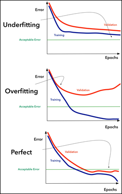
1. Overfitting: In this scenario, the model becomes too complex and learns the noise in the training data, resulting in high training error and poor generalization to new data.

As we can see in this image, the training loss (blue) decreases rapidly with an increasing number of iterations, while the validation loss (red) starts to increase after a certain point, indicating that the model is starting to overfit to the training data.
2. Underfitting: In this scenario, the model is too simple and does not capture the underlying patterns in the data, resulting in high training and validation errors.

As we can see in this image, the training loss (blue) decreases gradually with an increasing number of iterations, but the validation loss (red) remains high and does not decrease much, indicating that the model is too simple and is not capturing the patterns in the data.

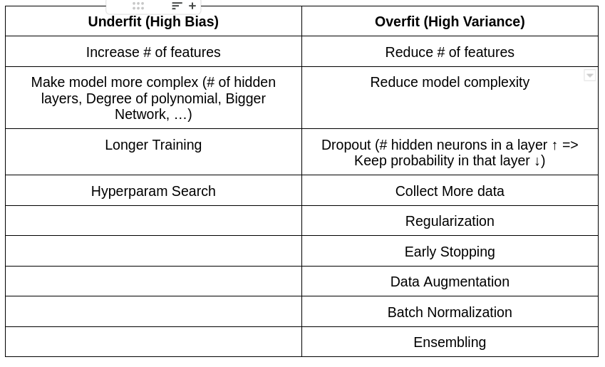
3) What’s the bias-variance trade-off? How’s this tradeoff related to overfitting and underfitting? How do you know that your model is high variance, low bias? What would you do in this case? How do you know that your model is low variance, high bias? What would you do in this case?

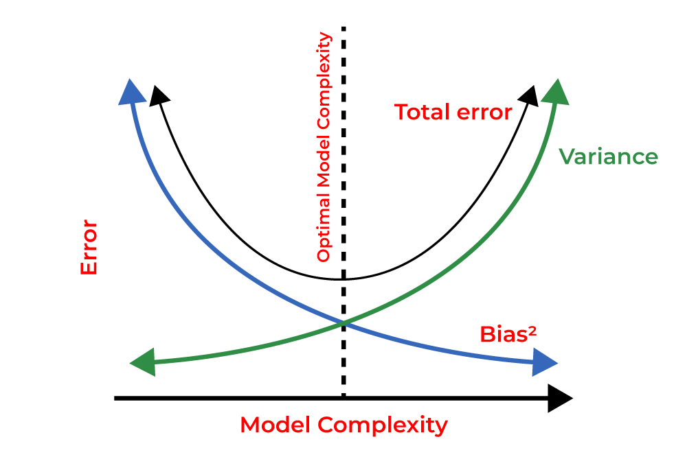
1. The bias-variance tradeoff is a fundamental concept in machine learning that deals with the tradeoff between the bias (underfitting) and variance (overfitting) of a model. It refers to the relationship between the model’s ability to capture the true underlying patterns in the data (bias) and its sensitivity to variations in the training data (variance). Understanding this tradeoff is essential for building models that generalize well to unseen data.

To explain the bias-variance tradeoff, let’s consider the following:

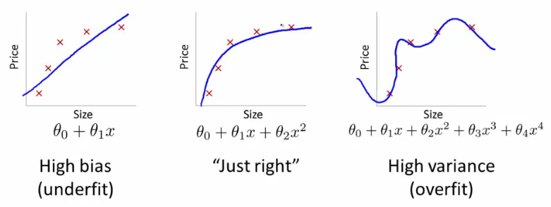
Bias: Bias measures the error introduced by approximating a real-world problem with a simplified model. A model with high bias tends to make strong assumptions or have limitations that prevent it from capturing complex patterns in the data. It can result in underfitting, where the model is too simple and fails to capture important relationships, leading to high training and test errors.

Variance: Variance measures the model’s sensitivity to fluctuations in the training data. A model with high variance is overly complex and captures noise or random variations in the training set. It performs well on the training data but fails to generalize to new, unseen data. This is known as overfitting, where the model becomes too specialized to the training data and fails to capture the underlying patterns of the problem.

The bias-variance tradeoff can be visualized as follows:
High Bias, Low Variance: Models with high bias and low variance are typically simple, making strong assumptions about the data. They tend to have low flexibility and may not capture complex relationships. These models can result in underfitting, where both the training and test errors are high.
Low Bias, High Variance: Models with low bias and high variance are often more complex and flexible, capturing fine-grained details in the training data. However, they are sensitive to variations in the training set and may overfit. These models can achieve low training error, but their performance on unseen data is poor, leading to high test error.

2. The bias-variance trade-off is directly related to overfitting and underfitting. When a model is underfitting, it has high bias and low variance. This means that the model is not complex enough to capture the underlying patterns in the data, and it is not able to generalize well to new data. On the other hand, when a model is overfitting, it has low bias and high variance. This means that the model is too complex and is fitting the training data too closely, resulting in poor generalization to new data.
3. You can tell that your model is high variance and low bias if it has a low training error but a high validation error. This indicates that the model is overfitting to the training data and is not able to generalize well to new data. In this case, you can try reducing the complexity of the model by simplifying the architecture, reducing the number of features, or increasing the regularization.
4. You can tell that your model is low variance and high bias if it has a high training error and a high validation error. This indicates that the model is not able to capture the underlying patterns in the data and is not complex enough to generalize well to new data. In this case, you can try increasing the complexity of the model by adding more features or increasing the depth of the neural network. It is important to monitor the model’s performance on a validation set and make small incremental changes to avoid overfitting.

4) Explain different methods for cross-validation. Why don’t we see more cross-validation in deep learning?

Cross-validation is a resampling technique used in machine learning to evaluate the performance of a model and estimate its generalization ability. It involves partitioning the available data into multiple subsets and iteratively training and testing the model on different combinations of these subsets. Here are some common methods for cross-validation:

1. K-Fold Cross-Validation: In k-fold cross-validation, the data is divided into k equally sized folds. The model is trained and evaluated k times, each time using a different fold as the validation set and the remaining folds as the training set. The performance metrics are then averaged over the k iterations to estimate the model’s performance.
2. Stratified K-Fold Cross-Validation: Stratified k-fold cross-validation is similar to k-fold cross-validation, but it preserves the class distribution in each fold. This is especially useful when dealing with imbalanced datasets, where the class proportions are uneven. Stratified sampling ensures that each fold has a representative distribution of classes, resulting in more reliable performance estimates.
3. Leave-One-Out Cross-Validation (LOOCV): LOOCV is a special case of k-fold cross-validation where k is equal to the number of instances in the dataset. For each iteration, the model is trained on all data except one instance, which is then used as the validation set. LOOCV provides a more exhaustive evaluation as each instance is used as a separate validation set, but it can be computationally expensive for large datasets.
4. Leave-P-Out Cross-Validation (LPOCV): LPOCV involves leaving out p data points from the training set and using them as the validation set. This process is repeated for all possible combinations of p points, resulting in multiple training-validation iterations. LPOCV allows for a more fine-grained evaluation but can be computationally expensive and may not be feasible for large datasets.
5. Time Series Cross-Validation: Time series data often exhibits temporal dependencies, making standard cross-validation methods inappropriate. Time series cross-validation techniques, such as forward chaining or rolling window validation, take into account the temporal ordering of the data. They train the model on past data and evaluate it on future data, simulating real-world scenarios where the model is deployed in a sequential manner.
6. Nested Cross-Validation: Nested cross-validation is used when hyperparameter tuning is involved. It combines an outer cross-validation loop with an inner loop for hyperparameter selection. The outer loop partitions the data into training and test sets, while the inner loop performs cross-validation on the training set to select the best hyperparameters. This nested approach provides more reliable performance estimates and helps avoid overfitting during hyperparameter tuning.

Cross-validation is less commonly used in deep learning because of the large size of the datasets and the high computational cost of training deep neural networks. In addition, deep learning models have a large number of hyperparameters, which makes it difficult to find the optimal hyperparameters using traditional cross-validation methods. Instead, researchers often use techniques such as early stopping, regularization, and hyperparameter tuning on a smaller validation set to prevent overfitting and improve model performance. However, cross-validation is still used in some cases, particularly when dealing with smaller datasets or when trying to compare different models.

https://neptune.ai/blog/cross-validation-in-machine-learning-how-to-do-it-right

5) What’s wrong with training and testing a model on the same data? Why do we need a validation set on top of a train set and a test set?

1. Training and testing a model on the same data can lead to overfitting, which means that the model will perform well on the training data but poorly on new, unseen data. This is because the model has essentially memorized the training data and has not learned to generalize to new data. Overfitting can also lead to poor performance when the model is deployed in the real world, as it will not be able to handle new situations that were not present in the training data.

The purpose of machine learning is to build models that can generalize well to new, unseen data. By testing a model on the same data used for training, we fail to assess its ability to generalize. The model may appear to perform well during testing, but its performance on real-world data could be significantly worse.

2. We need a validation set on top of a train set and a test set because the validation set allows us to tune the hyperparameters of the model without overfitting to the test data. The hyperparameters are settings that are chosen before training the model, such as the learning rate or the number of hidden layers in a neural network. The validation set is used to evaluate the model’s performance during training and to adjust the hyperparameters as necessary. Once the model has been trained and the hyperparameters have been optimized, the test set is used to evaluate the model’s final performance on new, unseen data. By separating the data into three sets (train, validation, and test), we can ensure that the model is able to generalize to new data and is not overfitting to the training or validation data.

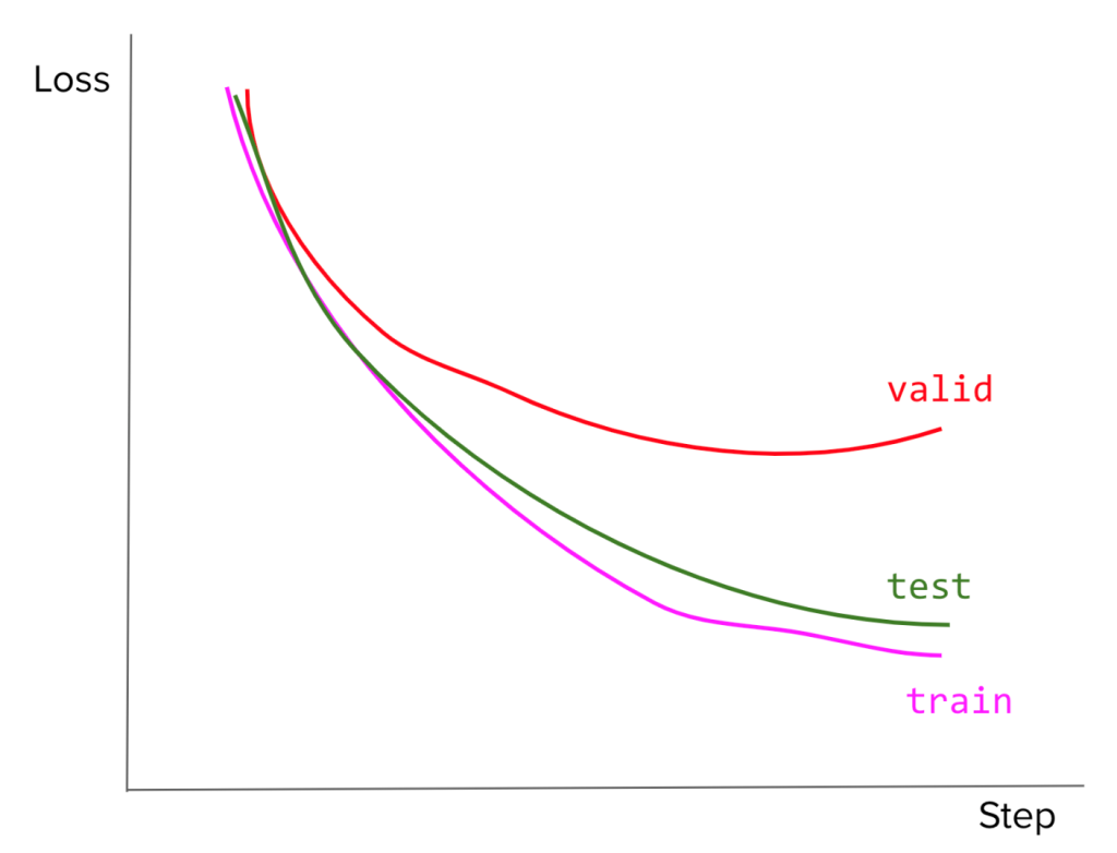
6) Your model’s loss curves on the train, valid, and test sets look like this. What might have been the cause of this? What would you do?

Diagnosing Unrepresentative Datasets
Learning curves can also be used to diagnose the properties of a dataset and whether it is relatively representative. An unrepresentative dataset means a dataset that may not capture the statistical characteristics relative to another dataset drawn from the same domain, such as between a train and a validation dataset. This can commonly occur if the number of samples in a dataset is too small or if certain characteristics are not adequately represented, relative to another dataset.
There are two common cases that could be observed; they are:
• Training dataset is relatively unrepresentative
• Validation dataset is relatively unrepresentative
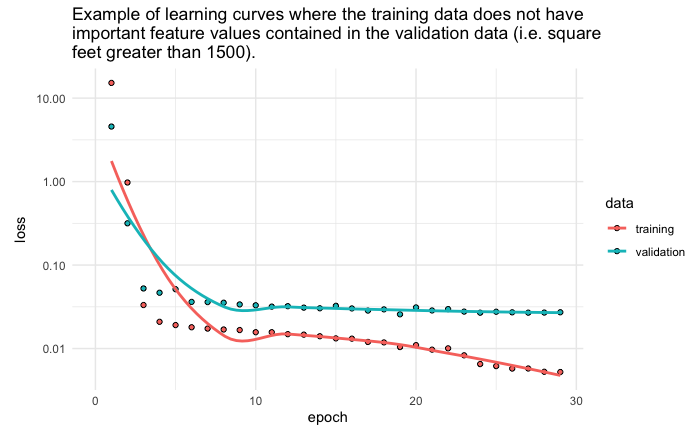
Unrepresentative train dataset
An unrepresentative training dataset means that the training dataset does not provide sufficient information to learn the problem, relative to the validation dataset used to evaluate it. This situation can be identified by a learning curve for training loss that shows improvement and similarly, a learning curve for validation loss that shows improvement, but a large gap remains between both curves. This can occur when
• The training dataset has too few examples as compared to the validation dataset.
• Training dataset contains features with less variance than the validation dataset.

Solution:
1. Add more observations. You may not have enough data to capture patterns present in both the training and validation data.
2. If using CNNs incorporate data augmentation to increase feature variability in the training data. ℹ️
3. Make sure that you are randomly sampling observations to use in your training and validation sets. If your data is ordered by some feature (i.e. neighborhood, class) then you validation data may have features not represented in your training data. ℹ️
4. Perform cross-validation so that all your data has the opportunity to be represented in both the training and validation sets. ℹ️
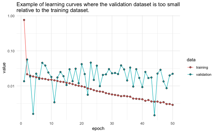
Unrepresentative validation dataset
An unrepresentative validation dataset means that the validation dataset does not provide sufficient information to evaluate the ability of the model to generalize. This may occur if the validation dataset has too few examples as compared to the training dataset. This case can be identified by a learning curve for training loss that looks like a good fit (or other fits) and a learning curve for validation loss that shows noisy movements and little or no improvement.

Solution:
1. Add more observations to your validation dataset.
2. If you are limited on the number of observations, perform cross-validation so that all your data has the opportunity to be represented in both the training and validation sets. ℹ️
It may also be identified by a validation loss that is lower than the training loss, no matter how many training iterations you perform. In this case, it indicates that the validation dataset may be easier for the model to predict than the training dataset. This can happen for various reason but is commonly associated with:
• Information leakage where a feature in the training data has direct ties to observations and responses in the validation data (i.e. patient ID).
• Poor sampling procedures where duplicate observations exist in the training and validation datasets.
• Validation dataset contains features with less variance than the training dataset.

Solution:
1. Check to make sure duplicate observations do not exists across training and validation datasets.
2. Check to make sure there is no information leakage across training and validation datasets.
3. Make sure that you are randomly sampling observations to use in your training and validation sets so that feature variance is consistent across both sets. ℹ️
4. Perform cross-validation so that all your data has the opportunity to be represented in both the training and validation s

7) What are the reasons why the validation loss is lower than the training loss?

Reason 1: L1 or L2 Regularization

Symptoms: validation loss is consistently lower than training loss, but the gap between them shrinks over time

Whether you’re using L1 or L2 regularization, you’re effectively inflating the error function by adding the model weights to it:

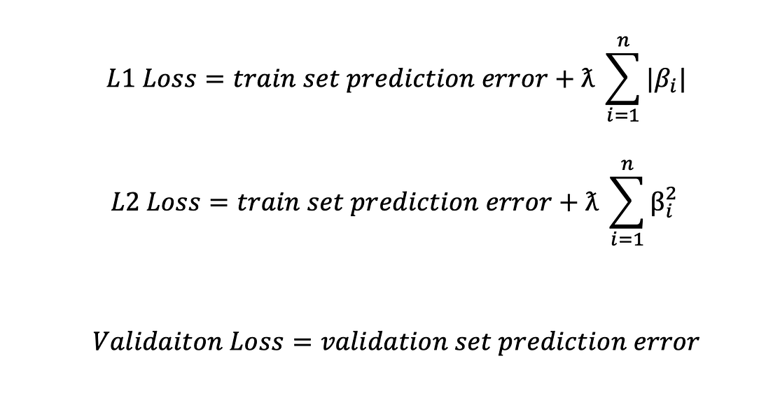
The regularization terms are only applied while training the model on the training set, inflating the training loss. During validation and testing, your loss function only comprises prediction error, resulting in a generally lower loss than the training set.

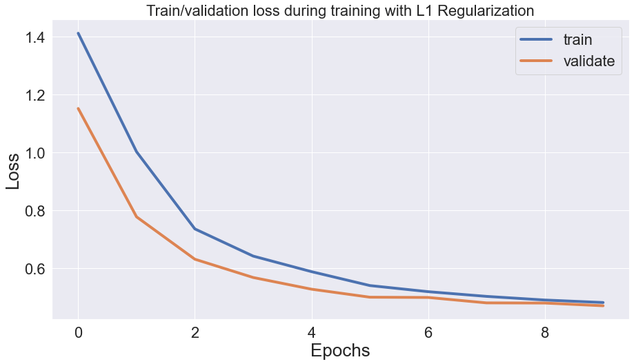
Notice how the gap between validation and train loss shrinks after each epoch. This is because as the network learns the data, it also shrinks the regularization loss (model weights), leading to a minor difference between validation and train loss.

However, the model is still more accurate on the training set.

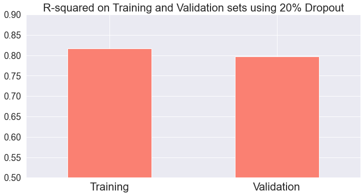
Let’s compare the R2 score of the model on the train and validation sets:

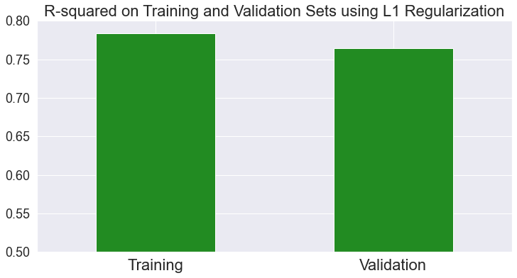
Notice that we’re not talking about loss and only focus on the model’s prediction on train and validation sets. As expected, the model predicts the train set better than the validation set.

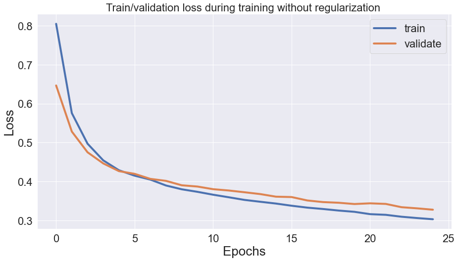
Reason 2: Dropout

Symptoms: validation loss is consistently lower than the training loss, the gap between them remains more or less the same size, and training loss has fluctuations.

Dropout penalizes model variance by randomly freezing neurons in a layer during model training. Like L1 and L2 regularization, dropout is only applicable during the training process and affects training loss, leading to cases where validation loss is lower than training loss.

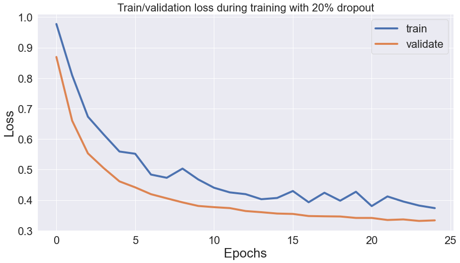
In this case, the model is more accurate on the training set as well:

Which is expected. Lower loss does not always translate to higher accuracy when you also have regularization or dropout in the network.

Reason 3: Training loss is calculated during each epoch, but validation loss is calculated at the end of each epoch

Symptoms: validation loss lower than training loss at first but has similar or higher values later on

Remember that each epoch is completed when all of your training data is passed through the network precisely once, and if you pass data in small batches, each epoch could have multiple backpropagations. Each backpropagation step could improve the model significantly, especially in the first few epochs when the weights are still relatively untrained.

As a result, you may get lower validation loss in the first few epochs when each backpropagation updates the model significantly.

Reason 4: Sheer luck! (Applicable to all ML models)

Symptoms: validation set has lower loss and higher accuracy than the training set. You also don’t have that much data.

Remember that noise is variations in the dependent variable that independent variables cannot explain. When you do the train/validation/test split, you may have more noise in the training set than in test or validation sets in some iterations. This makes the model less accurate on the training set if the model is not overfitting.

If you’re using it, this can be treated by changing the random seed in the train_test_split function (not applicable to time series analysis).

Note that this outcome is unlikely when the dataset is significant due to the law of large numbers.

Let’s conduct an experiment and observe the sensitivity of validation accuracy to random seed in train_test_split function. I’ll run model training and hyperparameter tuning in a for loop and only change the random seed in train_test_split and visualize the results:

for i in range(10):
    X_train, X_val, y_train, y_val = train_test_split(X, Y, test_size = 0.3, random_state = i)
    xg = XGBRegressor()
    grid_obj = GridSearchCV(xg, parameters, n_jobs=-1)
    grid_obj = grid_obj.fit(X_train, y_train)
    val_r2.append(r2_score(y_val, grid_obj.predict(X_val)))
    train_r2.append(r2_score(y_train, grid_obj.predict(X_train)))

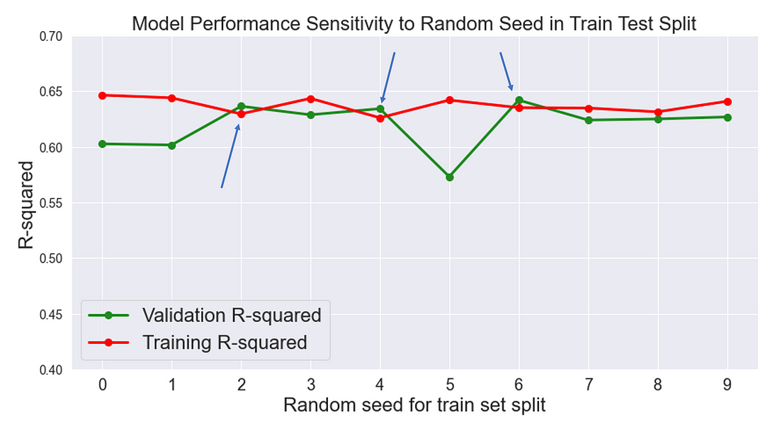
In 3 out of 10 experiments, the model had a slightly better R2 score on the validation set than the training set. In this case, changing the random seed to a value that distributes noise uniformly between validation and training set would be a reasonable next step.

There is more to be said about the plot. Data scientists usually focus on hyperparameter tuning and model selection while losing sight of simple things such as random seeds that drastically impact our results.

Check these links:

https://rstudio-conf-2020.github.io/dl-keras-tf/notebooks/learning-curve-diagnostics.nb.html

https://towardsdatascience.com/what-your-validation-loss-is-lower-than-your-training-loss-this-is-why-5e92e0b1747e

https://pyimagesearch.com/2019/10/14/why-is-my-validation-loss-lower-than-my-training-loss/embed/#?secret=sb4BKb9exw#?secret=8i3FrP9EX6

8) Your team is building a system to aid doctors in predicting whether a patient has cancer or not from their X-ray scan. Your colleague announces that the problem is solved now that they’ve built a system that can predict with 99.99% accuracy. How would you respond to that claim?

While achieving high accuracy on a classification task like predicting cancer is desirable, it is important to consider other factors that may affect the model’s performance. Here are some questions to ask in response to your colleague’s claim:
1. What was the size of the dataset used to train and test the model? A very small dataset may lead to overfitting and unrealistic high accuracy.
2. Did you use cross-validation or holdout validation to ensure that the model generalizes well to new data?
3. Are the classes balanced in the dataset? If one class is much more common than the other, a model that simply predicts the majority class can achieve high accuracy, even if it is not useful in practice.
4. Did you evaluate the model on a separate test set that the model has never seen before?
5. Did you consider other metrics, such as precision, recall, or F1-score, to evaluate the model’s performance? High accuracy alone may not be enough if the model makes many false positive or false negative predictions.
6. Did you analyze the model’s predictions and identify any biases or errors? For example, does the model perform well for certain types of cancer but poorly for others?
It’s important to carefully evaluate the performance of the model, taking into account these factors and more, before concluding that the problem is “solved”. It’s also important to recognize that predicting cancer is a complex problem that may require additional information beyond just X-ray scans, and that the model’s performance may vary in different populations or clinical settings.

9) What’s the benefit of F1 over accuracy? Can we still use F1 for a problem with more than two classes? How?

1. F1-score is a better metric than accuracy when the dataset is imbalanced, i.e., when there is a significant difference in the number of samples in each class. For instance, in a binary classification problem where the positive class is rare, a model that always predicts the negative class can have a high accuracy, but it is not useful in practice. F1-score takes into account both precision and recall, which are calculated based on true positives, false positives, and false negatives. Therefore, F1-score provides a more balanced evaluation of the model’s performance, especially in imbalanced datasets.
2. Yes, F1-score can be used for a problem with more than two classes.

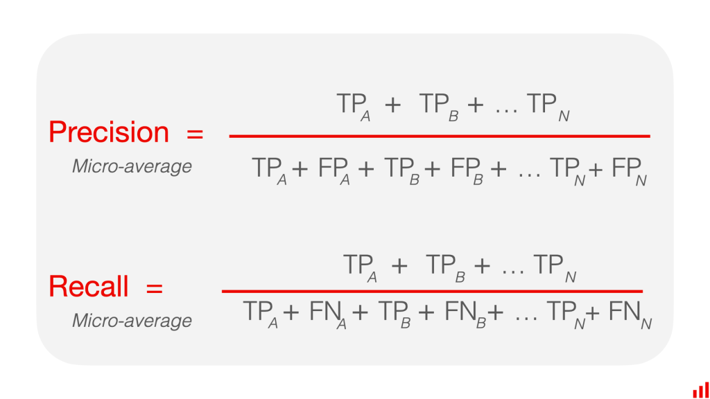
Micro-average aggregates the contributions of all classes to compute the average metric. This means that each example contributes equally to the final metric, regardless of the class it belongs to. To compute the micro-average precision, recall, and F1-score, we need to sum up the true positives, false positives, and false negatives across all classes, and then compute the metrics using these values.
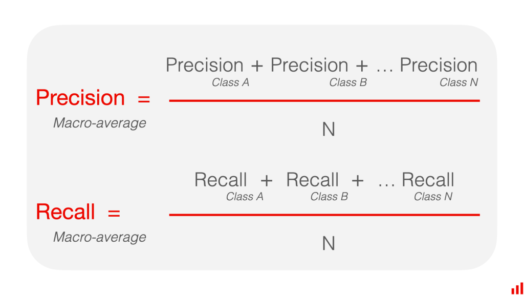
Macro-average, on the other hand, computes the average metric across all classes independently. This means that each class contributes equally to the final metric, regardless of its size. To compute the macro-average precision, recall, and F1-score, we need to compute the metric for each class separately, and then take the average of these values.
The main difference between micro-average and macro-average is that micro-average is influenced more by the performance on the larger classes, whereas macro-average is influenced equally by the performance on all classes. In other words, micro-average is better when the dataset is imbalanced and the majority class dominates the performance, while macro-average is better when all classes are equally important and we want to ensure that the model performs well on all of them.

Macro-averaging calculates each class’s performance metric (e.g., precision, recall) and then takes the arithmetic mean across all classes. So, the macro-average gives equal weight to each class, regardless of the number of instances.

Micro-averaging, on the other hand, aggregates the counts of true positives, false positives, and false negatives across all classes and then calculates the performance metric based on the total counts. So, the micro-average gives equal weight to each instance, regardless of the class label and the number of cases in the class.

Pros and cons

A suitable metric depends on the specific problem and the importance of each class or instance.

Macro-averaging treats each class equally.

• It can be useful when all classes are equally important, and you want to know how well the classifier performs on average across them. 
• It is also useful when you have an imbalanced dataset and want to ensure each class equally contributes to the final evaluation.

However, macro averaging can also distort the perception of performance. 

• For example, it can make the classifier look “worse” due to low performance in an unimportant and small class since it will still contribute equally to the overall score. 
• In the opposite scenario, it can disguise poor performance in the critical minority class when the overall number of classes is large. In this case, the “contribution” of each class is diluted. The classifier may still achieve high macro-averaged precision and recall by performing well on the majority classes but poorly on the minority class.

If classes have unequal importance, measuring precision and recall by class or weighing them by importance might be helpful.

Micro-averaging can be more appropriate when you want to account for the total number of misclassifications in the dataset. It gives equal weight to each instance and will have a higher score when the overall number of errors is low. (If this sounds like accuracy, it is because it is!)

However, micro-averaging can also overemphasize the performance of the majority class, especially when it dominates the dataset. In this case, micro-averaging can lead to inflated performance scores when the classifier performs well on the majority class but poorly (or very poorly) on the minority classes. If the class is small, you might not notice!

As a result, there is no single best metric. To choose the most suitable one, you need to consider the number of classes, their balance, and their relative importance.

Here is a numerical example:
Suppose we have a multi-class classification problem with 3 classes (Class A, Class B, and Class C), and the following confusion matrix:

	Predicted Class A	Predicted Class B	Predicted Class C
Actual Class A	10	5	0
Actual Class B	2	20	3
Actual Class C	1	3	15

To compute the micro-average and macro-average precision, recall, and F1-score, we would proceed as follows:
Micro-average:
• Precision = (10 + 20 + 15) / (10 + 5 + 0 + 20 + 2 + 3 + 1 + 3 + 15) = 0.76
• Recall = (10 + 20 + 15) / (10 + 5 + 2 + 20 + 3 + 1 + 3 + 15) = 0.76
• F1-score = 2 * (0.76 * 0.76) / (0.76 + 0.76) = 0.76
Macro-average:
• Precision = (10/13 + 20/28 + 15/18) / 3 = 0.77
• Recall = (10/15 + 20/25 + 15/19) / 3 = 0.75
• F1-score = 2 * (0.77 * 0.75) / (0.77 + 0.75) = 0.75

In this example, we can see that the micro-average and macro-average metrics are different due to the class imbalance. The micro-average F1-score is higher than the macro-average F1-score, which suggests that the model performs better on the larger classes (Class A and Class B) and worse on the smaller class (Class C). The macro-average F1-score gives equal importance to all classes and indicates that the overall performance of the model is moderate, with room for improvement in all classes.

Macro-averaging calculates each class’s performance metric (e.g., precision, recall) and then takes the arithmetic mean across all classes. So, the macro-average gives equal weight to each class, regardless of the number of instances.
Micro-averaging, on the other hand, aggregates the counts of true positives, false positives, and false negatives across all classes and then calculates the performance metric based on the total counts. So, the micro-average gives equal weight to each instance, regardless of the class label and the number of cases in the class.

In multi-class classification cases where each observation has a single label, the micro-F1, micro-precision, micro-recall, and accuracy share the same value (i.e., 0.76 in this example).

And this explains why the classification report only needs to display a single accuracy value since micro-F1, micro-precision, and micro-recall also have the same value.

micro-F1 = accuracy = micro-precision = micro-recall

10) Given a binary classifier that outputs the following confusion matrix. Calculate the model’s precision, recall, and F1. What can we do to improve the model’s performance?

	Predicted True	Predicted False
Actual True	30	20
Actual False	5	40

Based on the given confusion matrix:
• True Positives (TP) = 30
• False Positives (FP) = 5
• False Negatives (FN) = 20
• True Negatives (TN) = 40
Therefore, the number of positive examples is 30 + 20 = 50, and the number of negative examples is 5 + 40 = 45.

Precision, recall, and F1 can be calculated as follows:

Precision = True positives / (True positives + False positives) = 30 / (30 + 5) = 0.857
Recall (sensitivity) = True positives / (True positives + False negatives) = 30 / (30 + 20) = 0.6
F1-score = 2 * (precision * recall) / (precision + recall) = 2 * (0.857 * 0.6) / (0.857 + 0.6) = 0.706

2. To improve the model’s performance, we can try several approaches, including:
• Collect more data to balance the classes if possible.
• Try different algorithms or models that are better suited for imbalanced data, such as decision trees, random forests, or ensemble methods.
• Resample the data by oversampling the minority class or undersampling the majority class to achieve a more balanced dataset.
• Adjust the classification threshold to bias the classifier towards the minority class.
• Consider using cost-sensitive learning to assign different costs to misclassification errors in each class.

Not sure how to improve the precision and recall of your machine learning model? These tips and techniques are a great place to start.

1. Collect more data: Increasing the amount of training data can often improve the performance of a machine learning model, as the model will have more examples to learn from. This is particularly useful if the current dataset is small or imbalanced (e.g., there are significantly more negative cases than positive cases).
2. Fine-tune model hyperparameters: Hyperparameters are the settings that can be adjusted for a machine learning model. Fine-tuning these settings can often improve model performance. For example, increasing the regularization strength for a model may improve precision, while decreasing the regularization strength may improve recall.
3. Use a different machine learning algorithm: Different machine learning algorithms can have different trade-offs between precision and recall. For example, decision trees tend to have higher recall compared to precision, while support vector machines tend to have higher precision compared to recall. Experimenting with different algorithms can help find the one that works best for a particular task.
4. Implement class weights: If the positive and negative cases in the dataset are imbalanced (e.g., there are significantly more negative cases than positive cases), then the model may be biased towards the more prevalent class. Implementing class weights (i.e., giving more weight to the minority class) can help balance the precision and recall of the model.
5. Use ensembling: Ensembling is the process of combining the predictions of multiple models to improve the overall performance. Ensembling can often improve the precision and recall of the final model.
6. Use domain knowledge: Applying domain knowledge to the feature engineering process (i.e., the process of selecting and creating the input features used by the model) can help improve the precision and recall of the model. For example, if you are building a model to detect spam emails, using features that are specifically related to spam emails (e.g., the presence of certain words or phrases) may improve the model’s performance.
7. Use data augmentation: Data augmentation is the process of generating additional training data by applying transformations to the existing data. For example, if you are building a image classification model, you can generate additional data by applying rotations, translations, and other transformations to the existing images. This can help improve the generalization of the model and improve precision and recall.
8. Use feature selection: Feature selection is the process of selecting the most relevant features from a larger set of features. Using a smaller set of more relevant features can improve the precision and recall of the model, as the model will have less noise to learn from. There are several techniques for feature selection, such as wrapper methods and filter methods.
9. Use data balancing techniques: If the positive and negative cases in the dataset are imbalanced (e.g., there are significantly more negative cases than positive cases), then the model may be biased towards the more prevalent class. There are several techniques that can be used to balance the dataset, such as oversampling the minority class or undersampling the majority class. These techniques can help improve the precision and recall of the model.

11) Consider a classification where 99% of data belongs to class A and 1% of data belongs to class B. If your model predicts A 100% of the time, what would the F1 score be? Hint: The F1 score when A is mapped to 0 and B to 1 is different from the F1 score when A is mapped to 1 and B to 0. If we have a model that predicts A and B at a random (uniformly), what would the expected F1 be?

Assuming that class A is mapped to 1 and class B is mapped to 0, and the model predicts class A 100% of the time, then:
• Precision = TP / (TP + FP) = 0 / (0 + 0) = undefined
• Recall = TP / (TP + FN) = 0 / (0 + 1) = 0
• F1 Score = 2 * (Precision * Recall) / (Precision + Recall) = undefined
This is because Precision is undefined when there are no positive predictions, and F1 Score requires both Precision and Recall to be defined. In this case, the model is not making any positive predictions for class B, so there are no false positives, true positives, or precision. The model is also missing all positive examples for class B, so there are no true positives or recall. Therefore, the F1 Score is undefined.

we have a dataset of 1000 patients and we want to predict whether they have a rare disease called “X”. Out of these 1000 patients, only 10 actually have the disease, while the remaining 990 are healthy. What is the precision and recall value in the following cases: 1) a predictor predicts all samples as having disease X. 2)a predictor predicts all samples as not having disease X. 3) a predictor predicts have X and not have X at a random (uniformly)

Given:
• Total number of patients = 1000
• Number of patients having disease X = 10
• Number of patients not having disease X = 990
1. If the predictor predicts all samples as having disease X:
• True Positives (TP) = 10
• False Positives (FP) = 990
• True Negatives (TN) = 0
• False Negatives (FN) = 0
Precision = TP / (TP + FP) = 10 / (10 + 990) = 0.01 Recall = TP / (TP + FN) = 10 / (10 + 0) = 1.0
2. If the predictor predicts all samples as not having disease X:
• True Positives (TP) = 0
• False Positives (FP) = 0
• True Negatives (TN) = 990
• False Negatives (FN) = 10
Precision = TP / (TP + FP) = 0 / (0 + 0) = Undefined (division by zero) Recall = TP / (TP + FN) = 0 / (0 + 10) = 0.0
3. If the predictor predicts having X and not having X at random (uniformly):
• True Positives (TP) and False Positives (FP) will be randomly assigned, on average 10% of the total samples will be assigned TP and 90% will be assigned FP.
• True Negatives (TN) and False Negatives (FN) will also be randomly assigned, on average 99% of the total samples will be assigned TN and 1% will be assigned FN.
Precision = TP / (TP + FP) = (10% of 1000) / 1000 = 0.1 Recall = TP / (TP + FN) = (10% of 10) / 10 = 1.0

12) For logistic regression, why is log loss recommended over MSE (mean squared error)?

As you might know normally LogLoss also known as CrossEntropy Loss is used in training a logistic regression classification model. The formulas for the same is as below

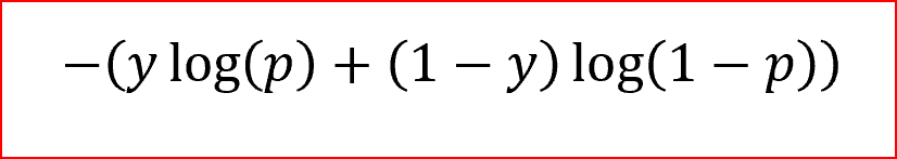
LogLoss Formula
In this y is the Actual value or the label
And p is the predicted value by the model.
This logloss is a convex function which means there exists only one local minima in the graph. And as with any other ML algorithm Gradient descent is used for optimization which is finding the best value of coefficients so that the value of the cost function is lowest. If you remember one of the main conditions for gradient descent is that the graph should have only one local minima on which it is iterating and trying to find optimal values.
Lets see this by plotting the log loss function. Breaking complicated things into smaller parts always makes it easier and quicker to understand. So let’s break things logloss function into parts. Depending on the value of yi it would be like this:

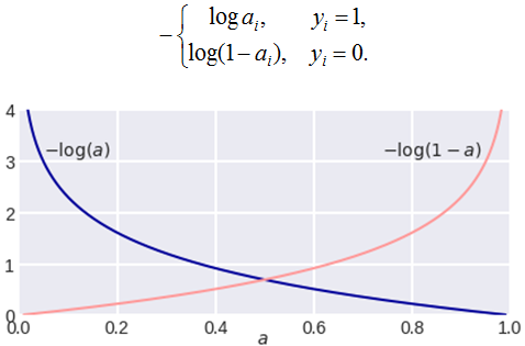
Plot of CrossEntropyLoss
Straightforward the local minima can be found at a=0.5. That’s why convex functions are important in gradient descents otherwise the algorithm would never find the exact local minima in a non-convex function as it contains more than one minima’s.
Now, lets move on to our main topic why MSE loss is not used in logistic regression. The whole context mentioned above is sufficient to understand the reason.

1. Non-Convex Nature

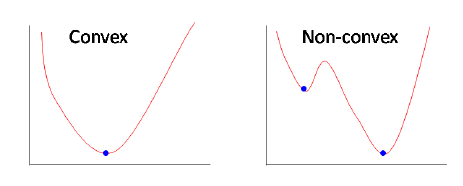
Convex vs Concave plots.
The graph of the Mean squared error function is non-convex for logistic regression. As we are putting dependent variable x in a non-linear sigmoid function. As discussed above gradient descent does not work for non-convex functions, logistic regression model would never be able to converge to optimal values.

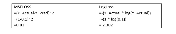
2. Penalization for wrong predictions.
   Okay if you don’t care about the optimizations and finding the best local minima and still want to use MSE Loss, it would still not work. why?
   If I ask you, What is the work of the cost function/Loss function?
   Basically, a cost function should be able to penalize the model in case of wrong predictions by outputting a higher loss value which will eventually result in a higher gradient value.
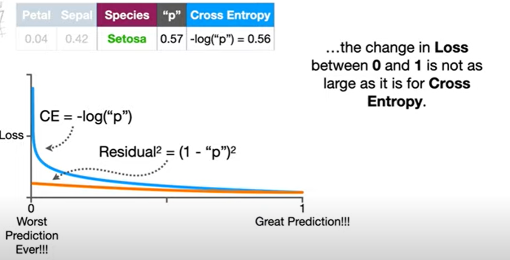
   But the Mean squared error used in logistic regression does not penalize the model in a great way. Ideally, MSELoss should be high for wrong class predictions but that does not happen, the reason being logistic regression is used for classification and all the predicted probability values lie between 0,1.
   Let’s say in a binary classification problem your model predicts a probability of class 1 as 0.1 (This is a clear example of misclassification).
   Here our Y_Actual=1 and Y_Pred=0.1
   Ideally, for a good cost function, the penalization/error value should be high. Let’s compare the Mean squared error and LogLoss for the same

1. The output of logistic regression is probabilities, not continuous values. Log loss is designed to evaluate the difference between predicted probabilities and actual classes, whereas MSE is designed to evaluate the difference between predicted and actual continuous values.
2. Log loss is a better metric for evaluating classification performance. It is particularly useful when dealing with imbalanced datasets, where the number of examples in each class is significantly different. Log loss takes into account the probability assigned to each class, so it can provide a more accurate evaluation of how well the model is performing.
3. Log loss is a convex function, which means that it has a unique global minimum. This makes it easier to optimize using gradient-based optimization algorithms.
4. Log loss has a probabilistic interpretation. It can be interpreted as the negative log-likelihood of the data under the logistic regression model, which means that minimizing log loss is equivalent to maximizing the likelihood of the data under the model.

https://medium.com/analytics-vidhya/understanding-the-loss-function-of-logistic-regression-ac1eec2838ce
https://towardsdatascience.com/why-not-mse-as-a-loss-function-for-logistic-regression-589816b5e03c

13) When should we use RMSE (Root Mean Squared Error) over MAE (Mean Absolute Error) and vice versa?

What is the difference between RMSE and MAE?
Whilst they both have the same goal of measuring regression model error, there are some key differences that you should be aware of:
1. RMSE is more sensitive to outliers
2. RMSE penalises large errors more than MAE due to the fact that errors are squared initially
3. MAE returns values that are more interpretable as it is simply the average of absolute error

RMSE is the square root of the mean of squared errors, which means it is more sensitive to large errors or outliers in the data. It can be useful when the target variable has a wide range of values and we want to penalize large errors more than small ones. RMSE is also commonly used when we want to compare the performance of different models on the same dataset.
MAE, on the other hand, is the mean of the absolute values of errors, which means it is less sensitive to outliers. It can be useful when the target variable has a small range of values and we want to penalize all errors equally. MAE is also simpler to calculate and easier to interpret than RMSE.
In summary, we should use RMSE when we want to penalize large errors more than small ones, and when we want to compare the performance of different models on the same dataset. We should use MAE when we want to penalize all errors equally, and when the target variable has a small range of values.

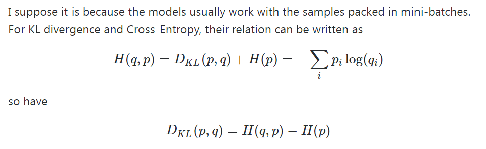
14) Show that the negative log-likelihood and cross-entropy are the same for binary classification tasks.

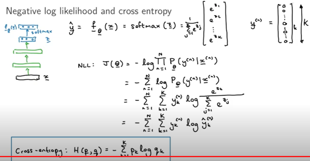
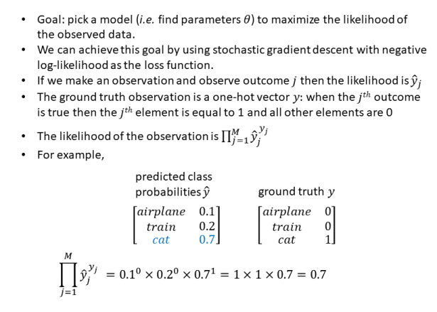
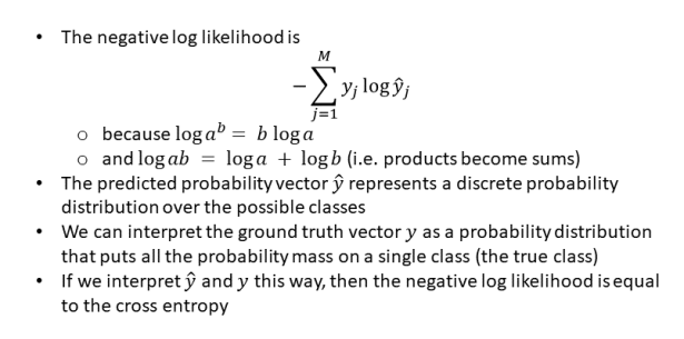
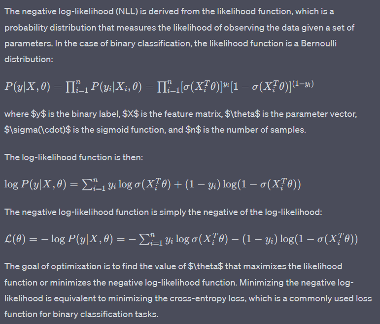
https://towardsdatascience.com/cross-entropy-negative-log-likelihood-and-all-that-jazz-47a95bd2e81

15) For classification tasks with more than two labels (e.g. MNIST with 10 labels), why is cross-entropy a better loss function than MSE?

First, Cross-entropy (or softmax loss, but cross-entropy works better) is a better measure than MSE for classification, because the decision boundary in a classification task is large (in comparison with regression). MSE doesn’t punish misclassifications enough but is the right loss for regression, where the distance between two values that can be predicted is small.
Second, from a probabilistic point of view, the cross-entropy arises as the natural cost function to use if you have a sigmoid or softmax nonlinearity in the output layer of your network, and you want to maximize the likelihood of classifying the input data correctly. If instead you assume the target is continuous and normally distributed, and you maximize the likelihood of the output of the net under these assumptions, you get the MSE (combined with a linear output layer). For classification, cross-entropy tends to be more suitable than MSE – the underlying assumptions just make more sense for this setting. That said, you can train a classifier with the MSE loss and it will probably work fine (although it does not play very nicely with the sigmoid/softmax nonlinearities, a linear output layer would be a better choice in that case). For regression problems, you would almost always use the MSE. Another alternative for classification is to use a margin loss, which basically amounts to putting a (linear) SVM on top of your network. ive for classification is to use a margin loss, which basically amounts to putting a (linear) SVM on top of your network.

Cross-entropy is a better loss function for classification tasks with more than two labels because it takes into account the probabilistic nature of the problem and penalizes the model for assigning low probability to the correct class. In contrast, MSE is not designed to handle classification tasks and does not account for the multi-class nature of the problem.
MSE measures the difference between the predicted and true values by squaring the error. However, in a multi-class classification problem, predicting the exact value for a label may not be necessary. Instead, the model needs to assign a probability distribution across all the possible labels and penalize the model for assigning low probabilities to the true label. Cross-entropy loss takes the predicted probabilities and calculates the difference between them and the true probabilities, with a larger penalty for larger differences.
In summary, cross-entropy loss is better suited for multi-class classification problems because it accounts for the probabilistic nature of the problem and provides a more accurate measure of the model’s performance.

15) Consider a language with an alphabet of 27 characters. What would be the maximal entropy of this language?

The maximal entropy of a language is achieved when all the characters are used with equal probability. In this case, since there are 27 characters, each character will be used with a probability of 1/27. The entropy of the language can be calculated using the formula:
H = -∑ p(x) log2 p(x)
where p(x) is the probability of character x and the sum is taken over all the characters in the alphabet.
For this language, the entropy would be:
H = -∑ (1/27) log2 (1/27) = -27(1/27)log2(1/27) = log2(27) ≈ 4.75 bits
Therefore, the maximal entropy of this language is approximately 4.75 bits.

16) A lot of machine learning models aim to approximate probability distributions. Let’s say P is the distribution of the data and Q is the distribution learned by our model. How do measure how close Q is to P?

https://towardsdatascience.com/entropy-cross-entropy-and-kl-divergence-17138ffab87b#:~:text=KL%20divergence%20is%20the%20relative,as%20the%20actual%20probability%20distribution.

There are various measures to quantify how close the distribution Q learned by the model is to the true distribution P of the data. One commonly used measure is the Kullback-Leibler (KL) divergence, also known as relative entropy.
The KL divergence is defined as the expectation of the logarithmic difference between P and Q:
KL(P||Q) = E[log(P(x)/Q(x))],
where x is a random variable, and the expectation is taken over all possible values of x according to the distribution P. KL divergence measures the difference between the true distribution P and the learned distribution Q. It is asymmetric and non-negative, which means that KL(P||Q) ≠ KL(Q||P) and KL(P||Q) ≥ 0.
Another measure to quantify the difference between P and Q is the Jensen-Shannon divergence (JS divergence), which is a symmetric and smoothed version of the KL divergence. The JS divergence is defined as:
JS(P,Q) = 1/2 * KL(P||(P+Q)/2) + 1/2 * KL(Q||(P+Q)/2),
where (P+Q)/2 is the average distribution between P and Q. JS divergence is a popular measure for comparing two probability distributions, especially in cases where Q is an empirical distribution obtained from a finite sample.

17) MPE (Most Probable Explanation) vs. MAP (Maximum A Posteriori) How do MPE and MAP differ? Give an example of when they would produce different results.

1. MPE (Most Probable Explanation) and MAP (Maximum A Posteriori) are both methods used in Bayesian inference to make predictions based on observed data and prior knowledge. However, they differ in the way they handle the prior knowledge. MPE aims to find the most likely explanation for the observed data, ignoring the prior knowledge. On the other hand, MAP combines the observed data with the prior knowledge by finding the maximum of the posterior probability distribution, which takes into account both the data and the prior.
2. Let’s consider an example where we want to predict the probability of rain tomorrow based on historical data. Suppose we have observed that it has rained on 60% of the days in the past, and we have a prior belief that rain is more likely during the winter months. We have two methods for predicting the probability of rain tomorrow: MPE and MAP.

Suppose the weather forecast predicts a low-pressure system moving in, which increases the chance of rain. Based on this information, MPE would simply predict that it will rain tomorrow, as this is the most likely explanation based on the observed data. However, MAP takes into account the prior belief that rain is more likely during the winter months, and may adjust the predicted probability of rain accordingly, resulting in a lower probability of rain tomorrow than what MPE predicts.

Let’s say we have a dataset of emails, and we want to build a model to classify them as either spam or not spam. We have a set of features for each email, such as the sender, subject, and content.
We can use MLE to estimate the parameters of a model that gives the probability of an email being spam given its features. Specifically, we can model the probability using a logistic regression, where the output is the probability of the email being spam and the inputs are the features of the email.
Once we have estimated the parameters of the model using MLE, we can use it to make predictions on new, unseen emails. For each email, we can calculate the probability of it being spam according to our model, and use a threshold (e.g., 0.5) to classify it as spam or not spam.
In contrast, MPE would give us the most likely explanation for each email, given the observed features. In this case, we could find the set of feature values that maximizes the probability of the email being classified as spam. This would give us the most probable explanation for why the email is classified as spam.

18) Suppose you want to build a model to predict the price of a stock in the next 8 hours and that the predicted price should never be off more than 10% from the actual price. Which metric would you use?

In this case, you would likely use the mean absolute percentage error (MAPE) as the evaluation metric. The MAPE measures the percentage difference between the predicted and actual values, which is appropriate for this scenario since you want to ensure that the predicted price is within 10% of the actual price. The formula for MAPE is:
MAPE = (1/n) * Σ(|(y_true – y_pred) / y_true|) * 100%
where y_true is the true value, y_pred is the predicted value, and n is the number of samples in the dataset. The MAPE is expressed as a percentage and represents the average percentage error between the predicted and actual values.

Refresher on Entropy:

In case you need a refresh on information entropy, here’s an explanation without any math.
Your parents are finally letting you adopt a pet! They spend the entire weekend taking you to various pet shelters to find a pet.
The first shelter has only dogs. Your mom covers your eyes when your dad picks out an animal for you. You don’t need to open your eyes to know that this animal is a dog. It isn’t hard to guess.
The second shelter has both dogs and cats. Again your mom covers your eyes and your dad picks out an email. This time, you have to think harder to guess which animal is that. You make a guess that it’s a dog, and your dad says no. So you guess it’s a cat and you’re right. It takes you two guesses to know for sure what animal it is.
The next shelter is the biggest one of them all. They have so many different kinds of animals: dogs, cats, hamsters, fish, parrots, cute little pigs, bunnies, ferrets, hedgehogs, chickens, and even exotic bearded dragons! There must be close to a hundred different types of pets. Now it’s really hard for you to guess which one your dad brings you. It takes you a dozen guesses to guess the right animal.
Entropy is a measure of the “spread out” in diversity. The more spread out the diversity, the header it is to guess an item correctly. The first shelter has very low entropy. The second shelter has a little bit higher entropy. The third shelter has the highest entropy.