
Prune unused Docker objects to alleviate low disk space on the filesystem root issues
2021-09-30Steps to Deploy Django with Postgres, Nginx, and Gunicorn on Ubuntu 18.04
2021-11-04Overview
Inverse transform sampling is a method for generating random numbers from any probability distribution by using its inverse cumulative distribution  . Recall that the cumulative distribution for a random variable X is
  . In what follows, we assume that our computer can, on-demand, generate independent realizations of a random variable
  uniformly distributed on [0,1].
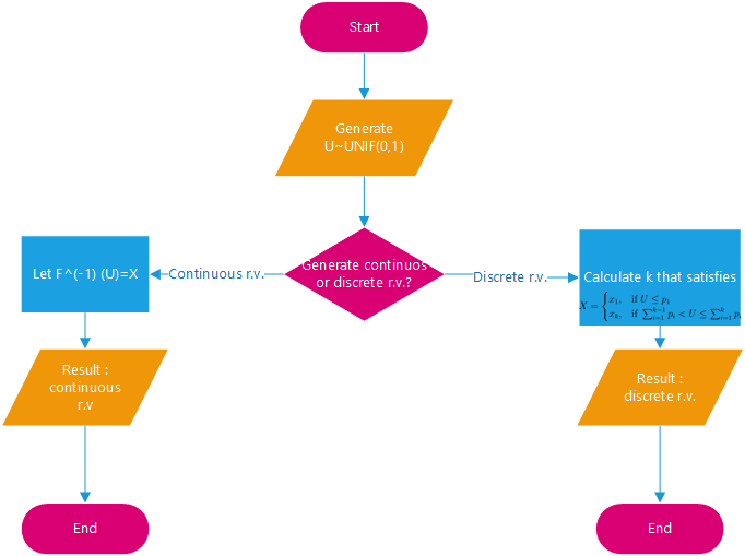
Algorithm
Continuous Distributions
Assume we want to generate a random variable  with cumulative distribution function (CDF)
  . The inverse transform sampling algorithm is simple:
1. Generate 
2. Let  .
.
Then, X will follow the distribution governed by the CDF , which was our desired result.
Note that this algorithm works in general but is not always practical. For example, inverting is easy if is an exponential random variable, but it is harder if is a Normal random variable.
Discrete Distributions
Now we will consider the discrete version of the inverse transform method. Assume that is a discrete random variable such that  . The algorithm proceeds as follows:
1. Generate
2. Determine the index k such that
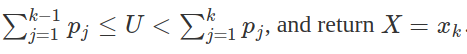
Notice that the second step requires a search.
Assume our random variable can take on any one of  values with probabilities
  . We implement the algorithm below, assuming these probabilities are stored in a vector called
 p.vec.
# note: this inefficient implementation is for pedagogical purposes
# in general, consider using the rmultinom() function
discrete.inv.transform.sample <- function( p.vec ) {
  U  <- runif(1)
  if(U <= p.vec[1]){
    return(1)
  }
  for(state in 2:length(p.vec)) {
    if(sum(p.vec[1:(state-1)]) < U && U <= sum(p.vec[1:state]) ) {
      return(state)
    }
  }
}
Continuous Example: Exponential Distribution
Assume Y is an exponential random variable with rate parameter λ=2. Recall that the probability density function is  , for y>0. First, we compute the
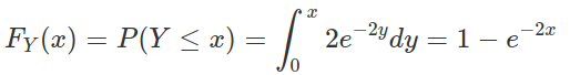
Solving for the inverse CDF, we get that
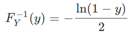
Using our algorithm above, we first generate U∼Unif(0,1), then set
We do this in the R code below and compare the histogram of our samples with the true density of Y.
# inverse transform sampling
num.samples <-  1000
U           <-  runif(num.samples)
X           <- -log(1-U)/2

# plot
hist(X, freq=F, xlab='X', main='Generating Exponential R.V.')
curve(dexp(x, rate=2) , 0, 3, lwd=2, xlab = "", ylab = "", add = T)
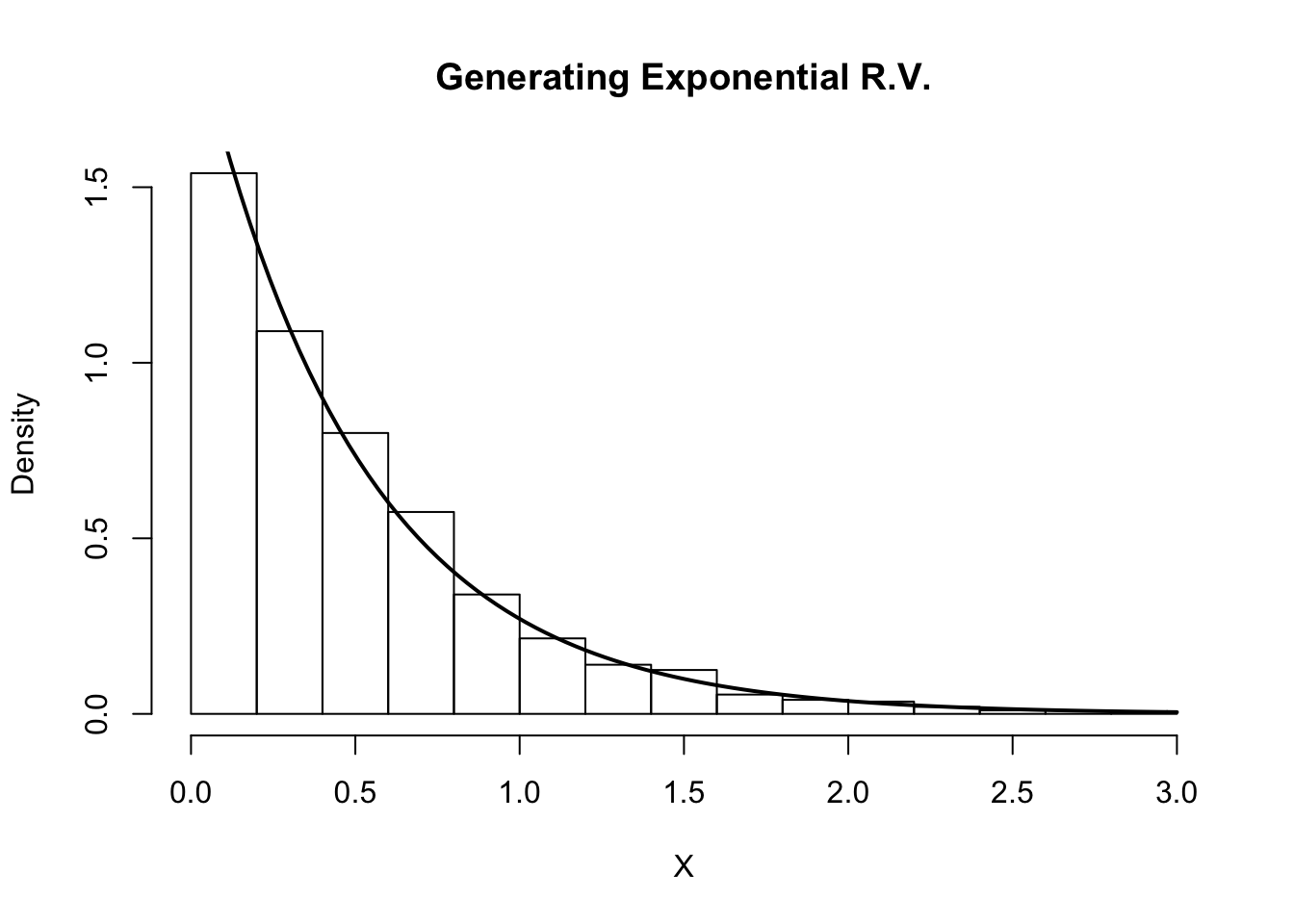
Indeed, the plot indicates that our random variables are following the intended distribution.
Python Example: Continuous case
First, we implement this method for generating continuous random variables. Suppose that we want to simulate a random variable X that follows the exponential distribution with mean λ (i.e. X~EXP(λ)). We know that the Probability Distribution Function (PDF) of the exponential distribution is

with the CDF as follows.

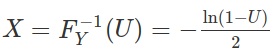
Then, we can write the inverse CDF as follows.

In Python, we can simply implement it by writing these lines of code as follows.
### Generate exponential distributed random variables given the mean
### and number of random variables
def exponential_inverse_trans(n=1,mean=1):
    U=uniform.rvs(size=n)
    X=-mean*np.log(1-U)
    actual=expon.rvs(size=n,scale=mean)

    plt.figure(figsize=(12,9))
    plt.hist(X, bins=50, alpha=0.5, label="Generated r.v.")
    plt.hist(actual, bins=50, alpha=0.5, label="Actual r.v.")
    plt.title("Generated vs Actual %i Exponential Random Variables" %n)
    plt.legend()
    plt.show()
    return X
We can try the code above by running some examples below. Note that the result might be different since we want to generate random variables.
cont_example1=exponential_inverse_trans(n=100,mean=4)
cont_example2=exponential_inverse_trans(n=500,mean=4)
cont_example3=exponential_inverse_trans(n=1000,mean=4)
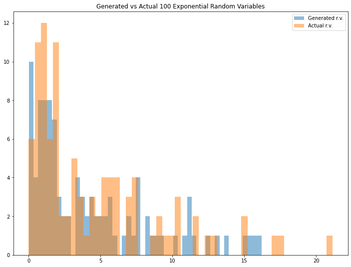
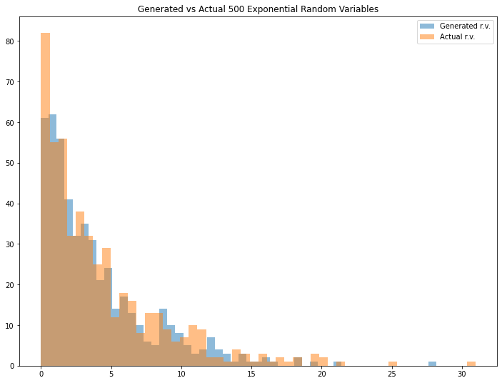
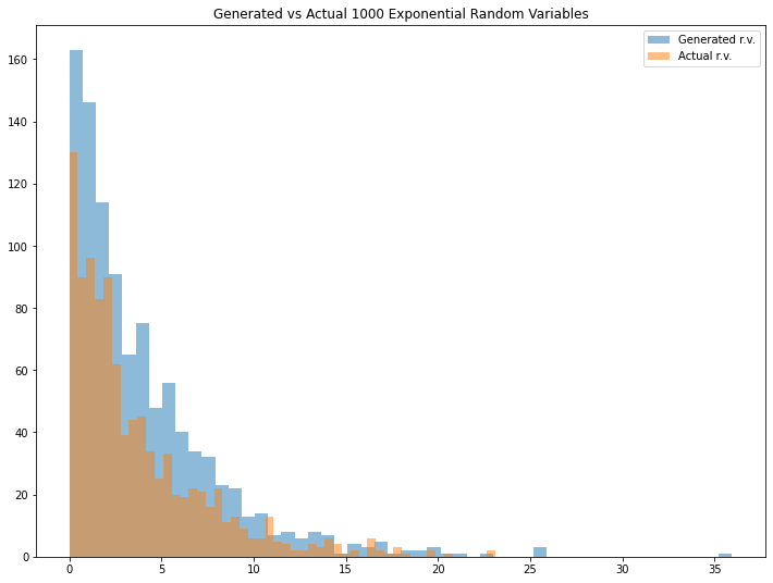
Looks interesting. We can see that the generated random variable has a pretty similar result if we compare it with the actual one. You can adjust the mean (Please note that the mean that I define for expon.rvs() function is a scale parameter in exponential distribution) and/or the number of generated random variables to see different results.
Discrete Example
In a discrete random variable case, suppose that we want to simulate a discrete random variable case X that follows the following distribution
 |  |
|---|---|
| 1 | 0.1 |
| 2 | 0.3 |
| 3 | 0.5 |
| 4 | 0.05 |
| 5 | 0.05 |
First, we write the function to generate the discrete random variable for one sample with these lines of code.
### Generate arbitary discrete distributed random variables given
### the probability vector
def discrete_inverse_trans(prob_vec):
    U=uniform.rvs(size=1)
    if U<=prob_vec[0]:
        return 1
    else:
        for i in range(1,len(prob_vec)+1):
            if sum(prob_vec[0:i])<U and sum(prob_vec[0:i+1])>U:
                return i+1
Then, we create a function to generate many random variable samples with these lines of code.
def discrete_samples(prob_vec,n=1):
    sample=[]
    for i in range(0,n):
        sample.append(discrete_inverse_trans(prob_vec))
    return np.array(sample)
We can run some examples below to see the results. Again, note that the result might be different since we want to generate random variables.
prob_vec=np.array([0.1,0.3,0.5,0.05,0.05])
numbers=np.array([1,2,3,4,5])
dis_example1=discrete_simulate(prob_vec, numbers, n=100)
dis_example2=discrete_simulate(prob_vec, numbers, n=500)
dis_example3=discrete_simulate(prob_vec, numbers, n=1000)
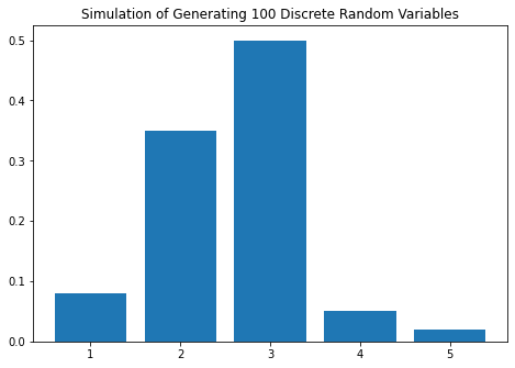
In[11]: dis_example1
Out[11]:
X Number of samples Empirical Probability Actual Probability
0 1 8 0.08 0.10
1 2 35 0.35 0.30
2 3 50 0.50 0.50
3 4 5 0.05 0.05
4 5 2 0.02 0.05
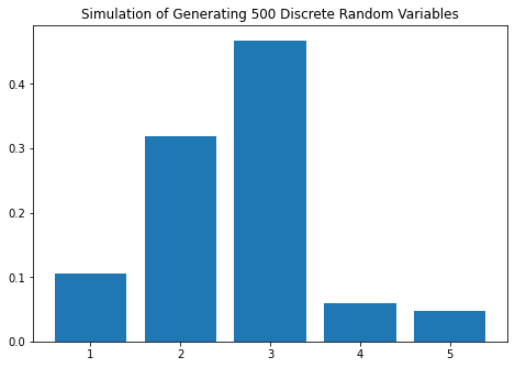
In[12]: dis_example2
Out[12]:
X Number of samples Empirical Probability Actual Probability
0 1 53 0.106 0.10
1 2 159 0.318 0.30
2 3 234 0.468 0.50
3 4 30 0.060 0.05
4 5 24 0.048 0.05
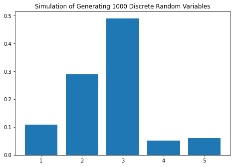
In[13]: dis_example3
Out[13]:
X Number of samples Empirical Probability Actual Probability
0 1 108 0.108 0.10
1 2 290 0.290 0.30
2 3 491 0.491 0.50
3 4 51 0.051 0.05
4 5 60 0.060 0.05
The result is interesting! We can see that the empirical probability is getting closer to the actual probability as we increase the number of random variable samples. Try to experiment with a different number of samples and/or different distribution to see different results.
References:
https://stephens999.github.io/fiveMinuteStats/inverse_transform_sampling.html