Implementations of Mutual Information (MI) and Entropy in Python

2017-06-14

Cythonize setup.py for several .pyx files

2017-06-17

Kernel Density Estimation (KDE) in Python

Nonparametric Density Estimation

In some cases, a data sample may not resemble a common probability distribution or cannot be easily made to fit the distribution. This is often the case when the data has two peaks (bimodal distribution) or many peaks (multimodal distribution). In this case, parametric density estimation is not feasible and alternative methods can be used that do not use a common distribution. Instead, an algorithm is used to approximate the probability distribution of the data without a pre-defined distribution, referred to as a nonparametric method.

The distributions will still have parameters but are not directly controllable in the same way as simple probability distributions. For example, a nonparametric method might estimate the density using all observations in a random sample, in effect making all observations in the sample “parameters.” Perhaps the most common nonparametric approach for estimating the probability density function of a continuous random variable is called kernel smoothing, or kernel density estimation, KDE for short.

A kernel is a mathematical function that returns a probability for a given value of a random variable. The kernel effectively smooths or interpolates the probabilities across the range of outcomes for a random variable such that the sum of probabilities equals one, a requirement of well-behaved probabilities. The kernel function weights the contribution of observations from a data sample based on their relationship or distance to a given query sample for which the probability is requested.

A parameter, called the smoothing parameter or the bandwidth, controls the scope, or window of observations, from the data sample that contributes to estimating the probability for a given sample. As such, kernel density estimation is sometimes referred to as a Parzen-Rosenblatt window, or simply a Parzen window, after the developers of the method.

Smoothing Parameter (bandwidth): Parameter that controls the number of samples or window of samples used to estimate the probability for a new point.

A large window may result in a coarse density with little details, whereas a small window may have too much detail and not be smooth or general enough to correctly cover new or unseen examples. The contribution of samples within the window can be shaped using different functions, sometimes referred to as basis functions, e.g. uniform normal, etc., with different effects on the smoothness of the resulting density function.

Basis Function (kernel): The function chosen used to control the contribution of samples in the dataset toward estimating the probability of a new point.

As such, it may be useful to experiment with different window sizes and different contribution functions and evaluate the results against histograms of the data.

In statistics, kernel density estimation (KDE) is a non-parametric way to estimate the probability density function of a random variable. Kernel density estimation is a fundamental data smoothing problem where inferences about the population are made, based on a finite data sample. In some fields such as signal processing and econometrics, it is also termed the Parzen–Rosenblatt window method, after Emanuel Parzen and Murray Rosenblatt, who are usually credited with independently creating it in its current form.

Definition

Let (x₁, x₂, …, x_n) be an independent and identically distributed sample drawn from some distribution with an unknown density ƒ. We are interested in estimating the shape of this function ƒ. Its kernel density estimator is

{\displaystyle {\hat {f}}_{h}(x)={\frac {1}{n}}\sum _{i=1}^{n}K_{h}(x-x_{i})={\frac {1}{nh}}\sum _{i=1}^{n}K{\Big (}{\frac {x-x_{i}}{h}}{\Big )},}

where K(•) is the kernel — a non-negative function that integrates to one and has mean zero — and h > 0 is a smoothing parameter called the bandwidth. A kernel with subscript h is called the scaled kernel and is defined as K_h(x) = 1/h K(x/h). Intuitively one wants to choose h as small as the data will allow; however, there is always a trade-off between the bias of the estimator and its variance. The choice of bandwidth is discussed in more detail below.

A range of kernel functions are commonly used: uniform, triangular, biweight, triweight, Epanechnikov, normal, and others. The Epanechnikov kernel is optimal in a mean square error sense,though the loss of efficiency is small for the kernels listed previously,^[4] and due to its convenient mathematical properties, the normal kernel is often used, which means K(x) = ϕ(x), where ϕ is the standard normal density function.

The construction of a kernel density estimate finds interpretations in fields outside of density estimation. For example, in thermodynamics, this is equivalent to the amount of heat generated when heat kernels (the fundamental solution to the heat equation) are placed at each data point locations x_i. Similar methods are used to construct discrete Laplace operators on point clouds for manifold learning.

Kernel density estimates are closely related to histograms but can be endowed with properties such as smoothness or continuity by using a suitable kernel. To see this, we compare the construction of histogram and kernel density estimators, using these 6 data points: x1 = −2.1, x2 = −1.3, x3 = −0.4, x4 = 1.9, x5 = 5.1, x6 = 6.2. For the histogram, first, the horizontal axis is divided into sub-intervals or bins which cover the range of the data. In this case, we have 6 bins each of width 2. Whenever a data point falls inside this interval, we place a box of height 1/12. If more than one data point falls inside the same bin, we stack the boxes on top of each other.

For the kernel density estimate, we place a normal kernel with a variance of 2.25 (indicated by the red dashed lines) on each of the data points x_i. The kernels are summed to make the kernel density estimate (solid blue curve). The smoothness of the kernel density estimate is evident compared to the discreteness of the histogram, as kernel density estimates converge faster to the true underlying density for continuous random variables.

Python Code:

First, we can construct a bimodal distribution by combining samples from two different normal distributions. Specifically, 300 examples with a mean of 20 and a standard deviation of 5 (the smaller peak), and 700 examples with a mean of 40 and a standard deviation of 5 (the larger peak). The means were chosen close together to ensure the distributions overlap in the combined sample.

The complete example of creating this sample with a bimodal probability distribution and plotting the histogram is listed below.

# example of a bimodal data sample
from matplotlib import pyplot
from numpy.random import normal
from numpy import hstack
# generate a sample
sample1 = normal(loc=20, scale=5, size=300)
sample2 = normal(loc=40, scale=5, size=700)
sample = hstack((sample1, sample2))
# plot the histogram
pyplot.hist(sample, bins=50)
pyplot.show()

Running the example creates the data sample and plots the histogram.

Note that your results will differ given the random nature of the data sample. Try running the example a few times.

We have fewer samples with a mean of 20 than samples with a mean of 40, which we can see reflected in the histogram with a larger density of samples around 40 than around 20.

Data with this distribution does not nicely fit into a common probability distribution, by design. It is a good case for using a nonparametric kernel density estimation method.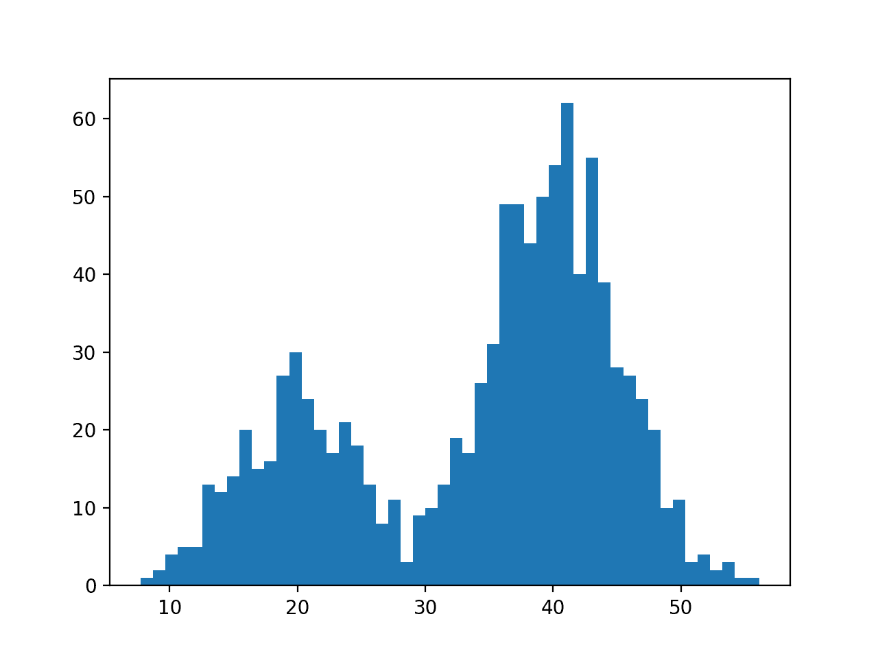 Histogram Plot of Data Sample With a Bimodal Probability Distribution

Histogram Plot of Data Sample With a Bimodal Probability Distribution

The scikit-learn machine learning library provides the KernelDensity class that implements kernel density estimation.

First, the class is constructed with the desired bandwidth (window size) and kernel (basis function) arguments. It is a good idea to test different configurations on your data. In this case, we will try a bandwidth of 2 and a Gaussian kernel.

The class is then fit on a data sample via the fit() function. The function expects the data to have a 2D shape with the form [rows, columns], therefore we can reshape our data sample to have 1,000 rows and 1 column.

...
# fit density
model = KernelDensity(bandwidth=2, kernel='gaussian')
sample = sample.reshape((len(sample), 1))
model.fit(sample)

We can then evaluate how well the density estimate matches our data by calculating the probabilities for a range of observations and comparing the shape to the histogram, just like we did for the parametric case in the prior section.

The score_samples() function on the KernelDensity will calculate the log probability for an array of samples. We can create a range of samples from 1 to 60, about the range of our domain, calculate the log probabilities, then invert the log operation by calculating the exponent or exp() to return the values to the range 0-1 for normal probabilities.

...
# sample probabilities for a range of outcomes
values = asarray([value for value in range(1, 60)])
values = values.reshape((len(values), 1))
probabilities = model.score_samples(values)
probabilities = exp(probabilities)

Finally, we can create a histogram with normalized frequencies and an overlay line plot of values to estimated probabilities.

...
# plot the histogram and pdf
pyplot.hist(sample, bins=50, density=True)
pyplot.plot(values[:], probabilities)
pyplot.show()

Tying this together, the complete example of kernel density estimation for a bimodal data sample is listed below.

# example of kernel density estimation for a bimodal data sample
from matplotlib import pyplot
from numpy.random import normal
from numpy import hstack
from numpy import asarray
from numpy import exp
from sklearn.neighbors import KernelDensity
# generate a sample
sample1 = normal(loc=20, scale=5, size=300)
sample2 = normal(loc=40, scale=5, size=700)
sample = hstack((sample1, sample2))
# fit density
model = KernelDensity(bandwidth=2, kernel='gaussian')
sample = sample.reshape((len(sample), 1))
model.fit(sample)
# sample probabilities for a range of outcomes
values = asarray([value for value in range(1, 60)])
values = values.reshape((len(values), 1))
probabilities = model.score_samples(values)
probabilities = exp(probabilities)
# plot the histogram and pdf
pyplot.hist(sample, bins=50, density=True)
pyplot.plot(values[:], probabilities)
pyplot.show()

Running the example creates the data distribution, fits the kernel density estimation model, then plots the histogram of the data sample and the PDF from the KDE model.

Note that your results will differ given the random nature of the data sample. Try running the example a few times.

In this case, we can see that the PDF is a good fit for the histogram. It is not very smooth and could be made more so by setting the “bandwidth” argument to 3 samples or higher. Experiment with different values of the bandwidth and the kernel function.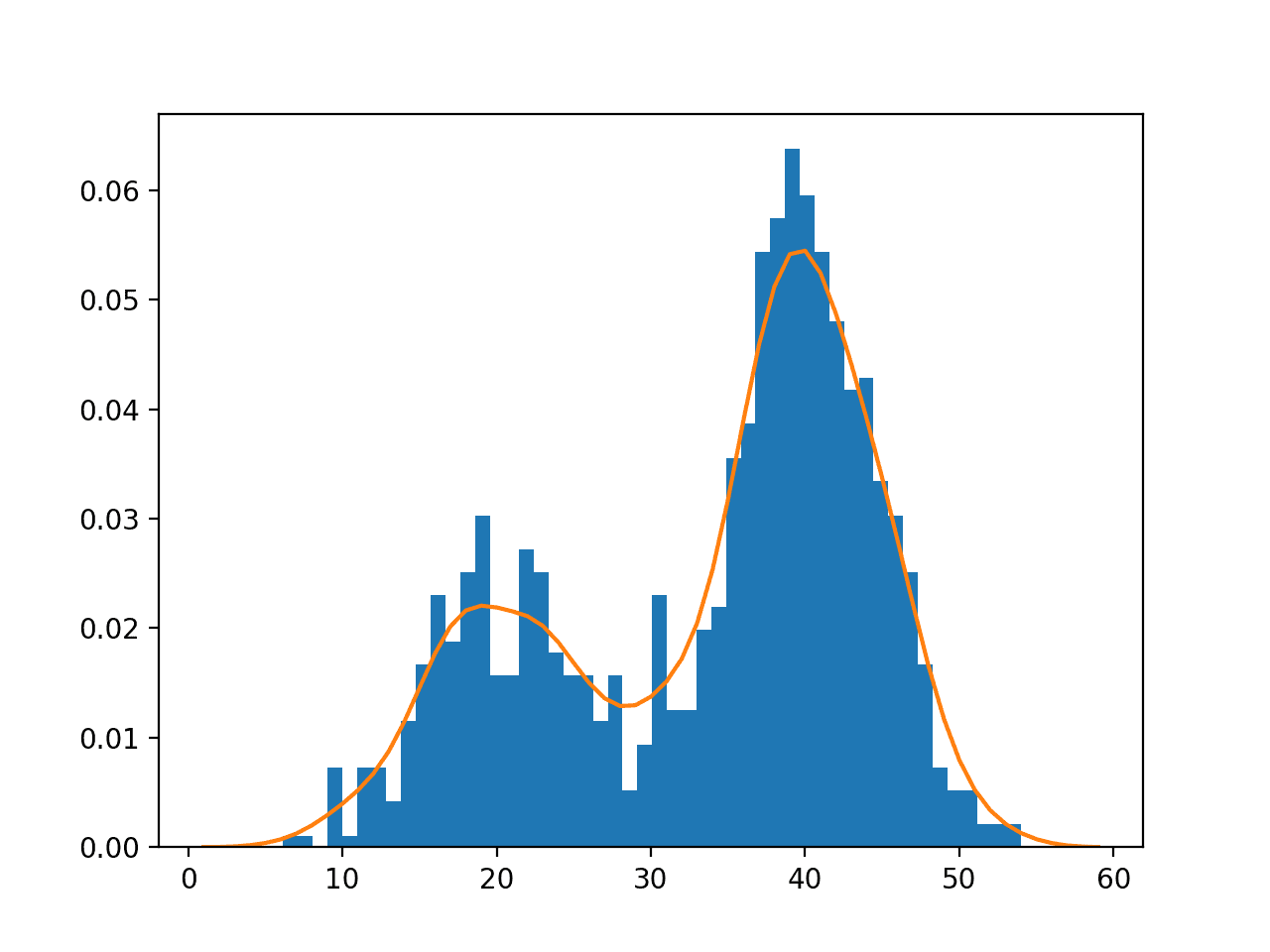 Histogram and Probability Density Function Plot Estimated via Kernel Density Estimation for a Bimodal Data Sample

Histogram and Probability Density Function Plot Estimated via Kernel Density Estimation for a Bimodal Data Sample

The KernelDensity class is powerful and does support estimating the PDF for multidimensional data.

Useful Links and Python Implementations:

Implementations of Mutual Information (MI) and Entropy in Python

Cythonize setup.py for several .pyx files

Kernel Density Estimation (KDE) in Python

Nonparametric Density Estimation

Definition

Related posts

Coursera Deep Learning Specialization Notes

Machine Learning for Big Data using PySpark with real-world projects

Leave a Reply Cancel reply