Understanding Micro, Macro, and Weighted Averages for Scikit-Learn metrics in multi-class classification with example

11 mins read

The F1 score, also known as the F-measure, stands as a widely-used metric to assess a classification model’s performance. When dealing with multi-class classification, we utilize averaging techniques to compute the F1 score, generating various average scores (macro, weighted, micro) in the classification report. This article delves into the significance of these averages, their calculation methods, and guidance on selecting the most suitable one for reporting purposes.

Basics

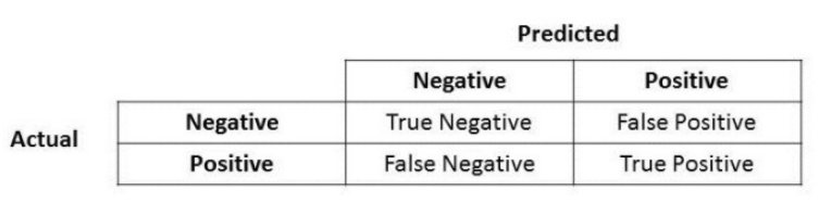
Anyone in the realm of Data Science is likely familiar with the concepts of Precision and Recall. These terms frequently surface when grappling with classification problems. If you’ve delved into Data Science, you’re probably aware of how relying solely on accuracy can often mislead when evaluating a model’s performance. However, I won’t delve into that here.

The formulas for Precision and Recall probably aren’t unfamiliar to you, but let’s have a quick review nonetheless:

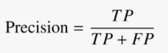
Precision

Layman definition: Of all the positive predictions I made, how many of them are truly positive?

Calculation: Number of True Positives (TP) divided by the Total Number of True Positives (TP) and False Positives (FP).

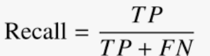
Recall

Layman definition: Of all the actual positive examples out there, how many of them did I correctly predict to be positive?

Calculation: Number of True Positives (TP) divided by the Total Number of True Positives (TP) and False Negatives (FN).

If you compare the formula for precision and recall, you will notice both look similar. The only difference is the second term of the denominator, where it is False Positive for precision but False Negative for recall.

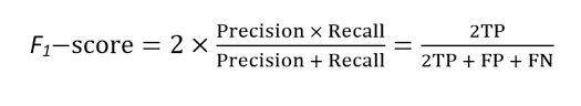
F1 Score

To evaluate model performance comprehensively, we should examine both precision and recall. The F1 score serves as a helpful metric that considers both of them.

Definition: Harmonic mean of precision and recall for a more balanced summarization of model performance.

Calculation:

These formulae can be used with only the Binary Classification problem (Something like Titanic on Kaggle where we have a ‘yes’ or ‘no’ or with problems with 2 labels for example Black or Red where we take one as 1 and the others as 0 ).

What about Multi-Class Problems?

If you encounter a classification challenge with three or more classes like Black, Red, Blue, White, etc., the earlier formulas for Precision and Recall might not seamlessly apply. However, determining accuracy shouldn’t pose a significant hurdle in such cases.

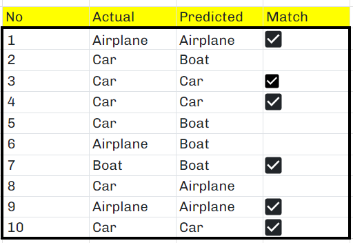
In order to demonstrate the averaging of F1 scores, let’s consider the following scenario within this tutorial’s context. Picture a scenario where we’ve trained an image classification model using a multi-class dataset comprising images falling into three classes: Airplane, Boat, and Car.

Now, let’s utilize this model to predict the classes of ten images from the test set. Here are the raw predictions:

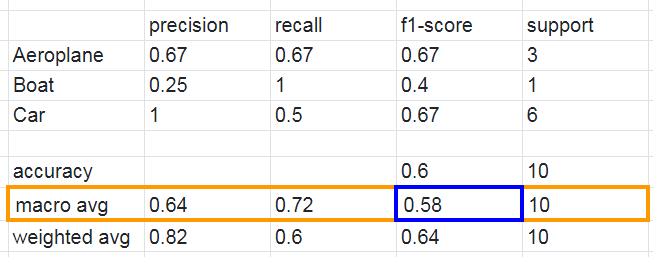
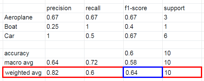
Upon running sklearn.metrics.classification_report, we get the following classification report:

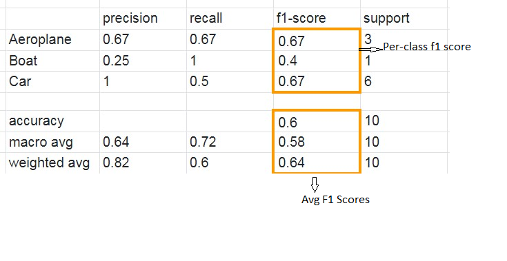
Our focus lies on the columns highlighted in orange, specifically the per-class scores (the scores for each class) and the average scores. In the provided scenario, it’s evident that the dataset is imbalanced, with only one out of ten test instances falling under the ‘Boat’ class. Consequently, relying solely on the proportion of correct matches (accuracy) might not effectively evaluate the model’s performance. Instead, let’s delve into the confusion matrix to gain a comprehensive understanding of the model’s predictions.

			Predicted
	Label	Airplane	Boat	Car
	Airplane	2	1	0
Actual	Boat	0	1	0
	Car	1	2	3

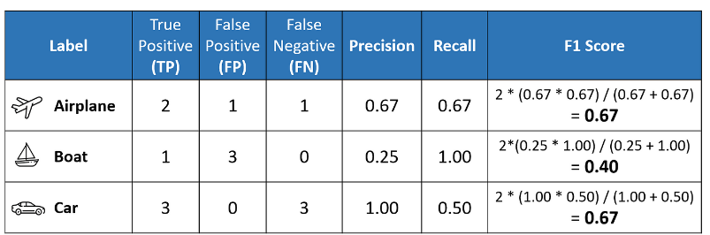
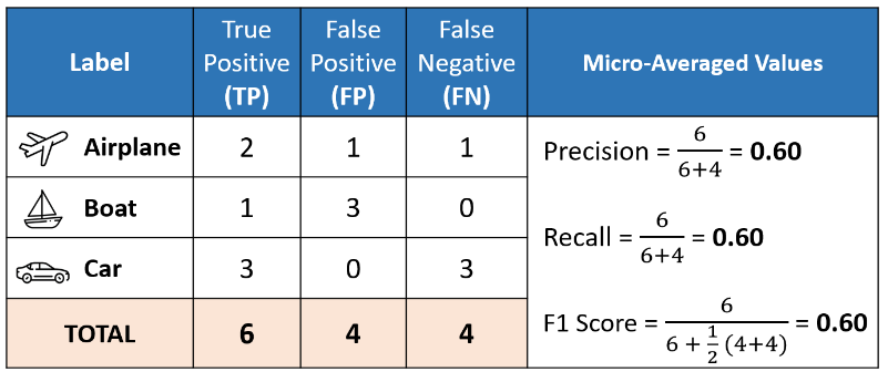
The confusion matrix above allows us to compute the critical values of True Positive (TP), False Positive (FP), and False Negative (FN), as shown below.

Label	True Positive (TP )	False Positive (FP )	False Negative (FN )
Airplane	2	1	1
Boat	1	3	0
Car	3	0	3

The above table sets us up nicely to compute the per-class values of precision, recall, and F1 score for each of the three classes. It is important to remember that in multi-class classification, we calculate the F1 score for each class in a One-vs-Rest (OvR) approach instead of a single overall F1 score as seen in binary classification. In this OvR approach, we determine the metrics for each class separately, as if there is a different classifier for each class. Here are the per-class metrics (with the F1 score calculation displayed):

However, instead of having multiple per-class F1 scores, it would be better to average them to obtain a single number to describe overall performance.

Now, let’s discuss the averaging methods that led to the three different average F1 scores in the classification report.

Macro Average

Macro averaging is perhaps the most straightforward among the numerous averaging methods. The macro-averaged F1 score (or macro F1 score) is computed by taking the arithmetic mean (aka unweighted mean) of all the per-class F1 scores. This method treats all classes equally regardless of their support values.

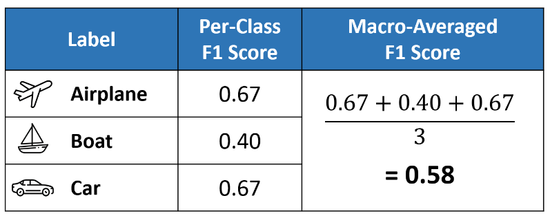
The value of 0.58 we calculated above matches the macro-averaged F1 score in our classification report.

Weighted Average

The weighted-averaged F1 score is calculated by taking the mean of all per-class F1 scores while considering each class’s support. Support refers to the number of actual occurrences of the class in the dataset. For example, the support value of 1 in Boat means that there is only one observation with an actual label of Boat. The ‘weight’ essentially refers to the proportion of each class’s support relative to the sum of all support values.

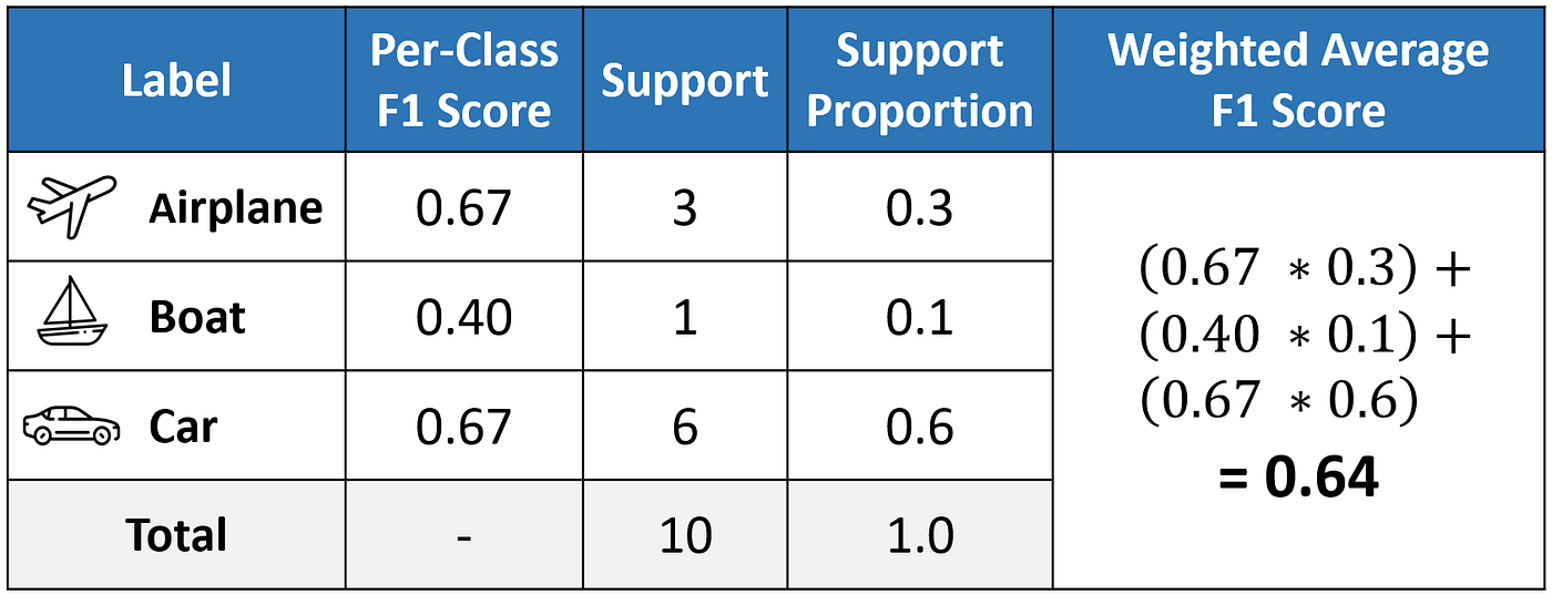
With weighted averaging, the output average would have accounted for the contribution of each class as weighted by the number of examples of that given class. The calculated value of 0.64 tallies with the weighted-averaged F1 score in our classification report.

Micro Average

Micro averaging computes a global average F1 score by counting the sums of the True Positives (TP), False Negatives (FN), and False Positives (FP). We first sum the respective TP, FP, and FN values across all classes and then plug them into the F1 equation to get our micro F1 score.

In the classification report, you might be wondering why our micro F1 score of 0.60 is displayed as ‘accuracy ’ and why there is NO row stating ‘micro avg’.

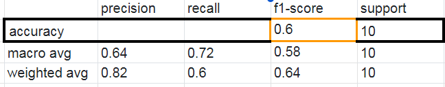
The reason is that micro-averaging essentially computes the proportion of correctly classified observations out of all observations. If we think about this, this definition is in fact what we use to calculate overall accuracy. Furthermore, if we were to do micro-averaging for precision and recall, we would get the same value of 0.60.

In multi-class classification scenarios where each observation carries a single label, the values for micro-F1, micro-precision, micro-recall, and accuracy align—such as the shared value of 0.60 in this example. Consequently, this elucidates why the classification report requires only one accuracy value, given the equivalence of micro-F1, micro-precision, and micro-recall.

micro-F1 = accuracy = micro-precision = micro-recall

A more detailed explanation of this observation can be found in this post.

Which average should we choose?

In the context of an imbalanced dataset where equal importance is attributed to all classes, opting for the macro average stands as a sound choice since it treats each class with equal significance. For instance, in our scenario involving the classification of airplanes, boats, and cars, employing the macro-F1 score would be appropriate.

However, when dealing with an imbalanced dataset and aiming to give more weight to classes with larger examples, the weighted average proves preferable. This approach adjusts the contribution of each class to the F1 average based on its size, offering a more balanced perspective.

In the case of a balanced dataset where a straightforward metric for overall performance, regardless of the class, is sought, accuracy becomes valuable—it essentially aligns with our micro F1 score.

Another example of calculating Precision and Recall for Multi-Class Problems

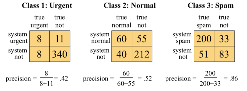
Let us first consider the situation. Assume we have a 3-class classification problem where we need to classify emails received as Urgent, Normal, or Spam. Now let us calculate Precision and Recall for this using the below methods:

MACRO AVERAGING

The Row labels (index) are output labels (system output) and Column labels (gold labels) depict actual labels. Hence,

• [urgent,normal]=10 means 10 normal(actual label) mails have been classified as urgent.
• [spam,urgent]=3 means 3 urgent(actual label) mails have been classified as spam

The mathematics isn’t tough here. Just a few things to consider:

• Summing over any row values gives us Precision for that class. Like precision_u=8/(8+10+1)=8/19=0.42 is the precision for class:Urgent

Similarly for precision_n(normal), precision_s(spam)

• Summing over any column gives us Recall for that class. Example:

recall_s=200/(1+50+200)=200/251=0.796. Similarly consider for recall_u (urgent) and recall_n(normal)

Now, to calculate the overall precision, average the three values obtained:

MICRO AVERAGING

Micro averaging follows the one-vs-rest approach. It calculates Precision and Recall separately for each class with True(Class predicted as Actual) and False(Classed predicted!=Actual class irrespective of which wrong class it has been predicted). The below confusion metrics for the 3 classes explain the idea better.

Now, we add all these metrics to produce the final confusion metric for the entire data i.e Pooled. Looking at cell [0,0] of Pooled matrix=Urgent[0,0] + Normal[0,0] + Spam[0,0]=8 + 60 + 200= 268

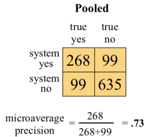
Now, using the old formula, calculating

precision= TruePositive(268)/(TruePositive(268) + FalsePositive(99))=0.73

Similarly, we can calculate Recall as well.

The calculations above illustrate how the Micro average gets influenced by the majority class (in this case, ‘Spam’), potentially masking the model’s performance across all classes—particularly the minority ones like ‘Urgent,’ which have fewer samples in the test data. On observation, it’s evident that the model’s performance for ‘Urgent’ is poor, with an actual precision of only 42%. Despite this, the overall number derived from micro-averaging could be misleading, showcasing a 70% precision. This is where macro-averaging proves advantageous over micro-averaging.

Summary

When you have a multiclass setting, the average parameter in the f1_score function needs to be one of these:

• ‘weighted’
• ‘micro’
• ‘macro’

The first one, ‘weighted’ calculates the F1 score for each class independently but when it adds them together uses a weight that depends on the number of true labels of each class:

therefore favoring the majority class.

‘micro’ uses the global number of TP, FN, and FP and calculates the F1 directly:

no favoring any class in particular.

Finally, ‘macro’ calculates the F1 separated by class but not using weights for the aggregation:

which results in a bigger penalization when your model does not perform well with the minority classes.

So:

• average=micro says the function to compute f1 by considering total true positives, false negatives, and false positives (no matter the prediction for each label in the dataset)
• average=macro says the function to compute f1 for each label, and returns the average without considering the proportion for each label in the dataset.
• average=weighted says the function to compute f1 for each label, and returns the average considering the proportion for each label in the dataset.

The one to use depends on what you want to achieve. If you are worried about class imbalance I would suggest using ‘macro’. However, it might be also worthwhile implementing some of the techniques available to tackle imbalance problems such as downsampling the majority class, upsampling the minority, SMOTE, etc.

Resources:

https://towardsdatascience.com/micro-macro-weighted-averages-of-f1-score-clearly-explained-b603420b292f

https://medium.com/data-science-in-your-pocket/calculating-precision-recall-for-multi-class-classification-9055931ee229

https://towardsdatascience.com/multi-class-metrics-made-simple-part-i-precision-and-recall-9250280bddc2

https://datascience.stackexchange.com/questions/40900/whats-the-difference-between-sklearn-f1-score-micro-and-weighted-for-a-mult