

A guide on PySpark Window Functions with Partition By
2022-02-17
Bulk Boto3 (bulkboto3): Python package for fast and parallel transferring a bulk of files to S3 based on boto3!
2022-03-28This post will provide you with an introduction to the Jacobian matrix and the Hessian matrix, including their definitions and methods for calculation. Additionally, the significance of the Jacobian determinant will be discussed. Lastly, the practical applications of these matrix types will be explored.
Table of Contents
What is the Jacobian matrix?
Example of the Jacobian matrix
Practice problems on finding the Jacobian matrix
Jacobian matrix determinant
The Jacobian and the invertibility of a function
Applications of the Jacobian matrix
What is the Hessian matrix?
Hessian matrix example
Practice problems on finding the Hessian matrix
Applications of the Hessian matrix
Bordered Hessian matrix
What is the Jacobian matrix?
The definition of the Jacobian matrix is as follows:
The Jacobian matrix is a matrix composed of the first-order partial derivatives of a multivariable function.
The formula for the Jacobian matrix is the following:
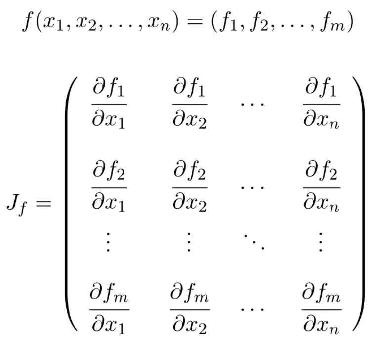
Therefore, Jacobian matrices will always have as many rows as vector components  and the number of columns will match the number of variables
  of the function.
As a curiosity, the Jacobian matrix was named after Carl Gustav Jacobi, an important 19th-century mathematician, and professor who made important contributions to mathematics, in particular to the field of linear algebra.
Example of the Jacobian matrix
Having seen the meaning of the Jacobian matrix, we are going to see step by step how to compute the Jacobian matrix of a multivariable function.
- Find the Jacobian matrix at the point (1,2) of the following function:

First of all, we calculate all the first-order partial derivatives of the function:


Now we apply the formula of the Jacobian matrix. In this case, the function has two variables and two vector components, so the Jacobian matrix will be a 2×2 square matrix:
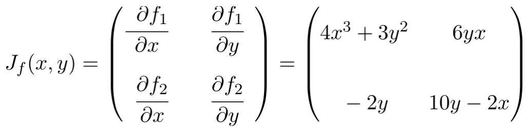
Once we have found the expression of the Jacobian matrix, we evaluate it at point (1,2):
![\displaystyle J_f(1,2)=\begin{pmatrix} 4\cdot 1^3+3\cdot 2^2 & 6\cdot 2 \cdot 1 \\[3ex] -2\cdot 2 & 10\cdot 2-2 \cdot 1 \end{pmatrix}](https://www.algebrapracticeproblems.com/wp-content/ql-cache/quicklatex.com-03c40ce3b3428c451dde68c4cb83d776_l3.svg "Rendered by QuickLaTeX.com")
And finally, we perform the operations:
![\displaystyle J_f(1,2)=\begin{pmatrix}16&12\\[3ex]-4&18\end{pmatrix}](https://www.algebrapracticeproblems.com/wp-content/ql-cache/quicklatex.com-8ad9612ae741a0727da116b0db9cfacc_l3.svg "Rendered by QuickLaTeX.com")
Once you have seen how to find the Jacobian matrix of a function, you can practice with several exercises solved step by step.
Examples:
Problem 1
Compute the Jacobian matrix at the point (0, -2) of the following vector-valued function with 2 variables:

Solution
The function has two variables and two vector components so the Jacobian matrix will be a square matrix of order 2:
Once we have calculated the expression of the Jacobian matrix, we evaluate it at the point (0, -2):
^2 & 2\cdot (-2) \cdot 0 \end{pmatrix}](https://www.algebrapracticeproblems.com/wp-content/ql-cache/quicklatex.com-f857e1b78007825da717d0bb1b1fa96a_l3.svg "Rendered by QuickLaTeX.com")
And finally, we perform all the calculations:
![\displaystyle \bm{J_f(0,-2)}=\begin{pmatrix} \bm{-2} & \bm{1} \\[1.5ex] \bm{4} & \bm{0} \end{pmatrix}](https://www.algebrapracticeproblems.com/wp-content/ql-cache/quicklatex.com-19f4d7e412b65625bc843152001d0ecf_l3.svg "Rendered by QuickLaTeX.com")
Problem 2
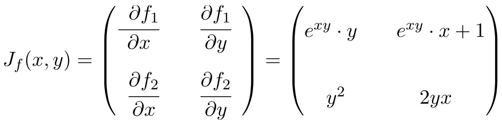
Calculate the Jacobian matrix of the following 2-variable function at the point (2, -1):

Solution
First, we apply the formula of the Jacobian matrix:
![\displaystyle J_f(x,y)=\begin{pmatrix}\cfrac{\phantom{5}\partial f_1}{\partial x}\phantom{5} & \phantom{5}\cfrac{\partial f_1}{\partial y}\phantom{5} \\[3ex] \cfrac{\partial f_2}{\partial x} & \cfrac{\partial f_2}{\partial y}\end{pmatrix} = \begin{pmatrix} \vphantom{\cfrac{\partial f_2}{\partial x}}3x^2y^2-10xy^2& 2x^3y-10x^2y \\[3ex] \vphantom{\cfrac{\partial f_2}{\partial x}} -3y^3 & 6y^5-9y^2x \end{pmatrix}](https://www.algebrapracticeproblems.com/wp-content/ql-cache/quicklatex.com-95d47cf9042d34448668364a91e52663_l3.svg "Rendered by QuickLaTeX.com")
Then we evaluate the Jacobian matrix at the point (2, -1):
![\displaystyle J_f(2,-1)=\begin{pmatrix} 3\cdot 2^2\cdot (-1)^2-10\cdot 2 \cdot (-1)^2\phantom{5} & \phantom{5}2\cdot 2^3\cdot (-1)-10\cdot 2^2\cdot (-1) \\[4ex] -3(-1)^3 & 6\cdot (-1)^5-9\cdot (-1)^2\cdot 2 \end{pmatrix}](https://www.algebrapracticeproblems.com/wp-content/ql-cache/quicklatex.com-e4cb42816012668ce5b379d5208d60d1_l3.svg "Rendered by QuickLaTeX.com")
So the solution to the problem is:
![\displaystyle \bm{J_f(1,2)}=\begin{pmatrix} \bm{-8} & \bm{24} \\[1.5ex] \bm{3} & \bm{-24} \end{pmatrix}](https://www.algebrapracticeproblems.com/wp-content/ql-cache/quicklatex.com-363e8856b5c9817179ebe6d8124d532b_l3.svg "Rendered by QuickLaTeX.com")
Problem 3
Determine the Jacobian matrix at the point (2, -2,2) of the following function with 3 variables:

Solution
In this case, the function has three variables and two scalar functions, therefore, the Jacobian matrix will be a rectangular 2×3 dimension matrix:
![\displaystyle J_f(x,y,z)= \begin{pmatrix}\cfrac{\phantom{5}\partial f_1}{\partial x}\phantom{5} & \phantom{5}\cfrac{\partial f_1}{\partial y}\phantom{5} & \phantom{5}\cfrac{\partial f_1}{\partial z}\phantom{5} \\[3ex] \cfrac{\partial f_2}{\partial x} & \cfrac{\partial f_2}{\partial y} &\cfrac{\partial f_2}{\partial z}\end{pmatrix}](https://www.algebrapracticeproblems.com/wp-content/ql-cache/quicklatex.com-cfd046d4ea24347650420c4beadac55b_l3.svg "Rendered by QuickLaTeX.com")
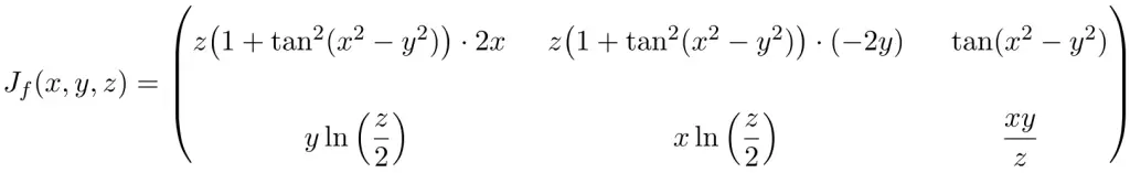
Once we have the Jacobian matrix of the multivariable function, we evaluate it at the point (2, -2,2):
![\displaystyle J_f(2,-2,2)= \begin{pmatrix} \vphantom{\cfrac{\partial f_2}{\partial x}}2\bigl(1+\tan^2 (2^2-(-2)^2)\bigr) \cdot 2\cdot 2 & 2\bigl(1+\tan^2 (2^2-(-2)^2)\bigr) \cdot (-2\cdot (-2)) & \tan (2^2-(-2)^2)\\[3ex] \vphantom{\cfrac{\partial f_2}{\partial x}} \displaystyle -2\ln \left( \frac{2}{2} \right) & \displaystyle 2\ln \left( \frac{2}{2} \right) &\displaystyle \frac{2\cdot (-2)}{2} \right)\end{pmatrix}](https://www.algebrapracticeproblems.com/wp-content/ql-cache/quicklatex.com-c6d5458ea6b5f32578758f33c4089b5e_l3.svg "Rendered by QuickLaTeX.com")
We perform all the calculations:
![\displaystyle J_f(2,-2,2)= \begin{pmatrix} \vphantom{\cfrac{\partial f_2}{\partial x}}2\bigl(1+\tan^2 (0)\bigr) \cdot 4 \phantom{5} & 2\bigl(1+\tan^2 (0)\bigr) \cdot 4 & \phantom{5}\tan (0)\\[3ex] \vphantom{\cfrac{\partial f_2}{\partial x}} -2\cdot 0 & 2\cdot 0 &-2 \right)\end{pmatrix}](https://www.algebrapracticeproblems.com/wp-content/ql-cache/quicklatex.com-8294403bbf8ddb5843652744cd5bf2d3_l3.svg "Rendered by QuickLaTeX.com")
![\displaystyle \bm{J_f(2,-2,2)=} \begin{pmatrix}\bm{8} & \bm{8} & \bm{0} \\[2ex] \bm{0} & \bm{0} &\bm{-2} \right)\end{pmatrix}](https://www.algebrapracticeproblems.com/wp-content/ql-cache/quicklatex.com-eaeea41806cc90582627e0c77921826c_l3.svg "Rendered by QuickLaTeX.com")
Problem 4
Find the Jacobian matrix of the following multivariable function at the point (π, π):

Solution
In this case, the function has two variables and vector components, therefore, the Jacobian matrix will be a rectangular matrix of size 3×2:
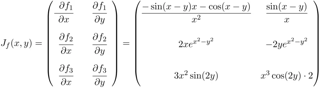
Secondly, we evaluate the Jacobian matrix at the point (π, π):
![\displaystyle J_f(\pi,\pi)= \begin{pmatrix} \displaystyle \vphantom{\cfrac{\partial f_3}{\partial y}}\frac{-\sin(\pi-\pi)\pi-\cos(\pi-\pi)}{\pi^2} & \displaystyle\frac{\sin (\pi- \pi)}{\pi} \\[3ex] \vphantom{\cfrac{\partial f_3}{\partial y}}2\pi e^{\pi^2-\pi^2} & -2\pi e^{\pi^2-\pi^2} \\[3ex] \vphantom{\cfrac{\partial f_3}{\partial y}} 3\pi^2\sin(2\pi) & \pi^3 \cos(2\pi)\cdot 2 \end{pmatrix}](https://www.algebrapracticeproblems.com/wp-content/ql-cache/quicklatex.com-2f1326efe7869f8bb8494c26ffff799f_l3.svg "Rendered by QuickLaTeX.com")
We compute all the operations:
![\displaystyle J_f(\pi,\pi)= \begin{pmatrix} \displaystyle \vphantom{\cfrac{\partial f_3}{\partial y}}\displaystyle\frac{-0-1}{\pi^2} & \displaystyle\frac{0}{\pi} \\[3ex] \vphantom{\cfrac{\partial f_3}{\partial y}}2\pi e^{0} & -2\pi e^{0} \\[3ex] \vphantom{\cfrac{\partial f_3}{\partial y}} 3\pi^2\cdot 0 & \pi^3 \cdot 1 \cdot 2 \end{pmatrix}](https://www.algebrapracticeproblems.com/wp-content/ql-cache/quicklatex.com-f1ef3124d6f462b14adf6b3e0d0e6a12_l3.svg "Rendered by QuickLaTeX.com")
So the Jacobian matrix of the vector-valued function at this point is:
![\displaystyle \bm{J_f(\pi,\pi)=} \begin{pmatrix}\displaystyle -\frac{\bm{1}}{\bm{\pi^2}} & \bm{0} \\[3ex] \bm{2\pi} & \bm{-2\pi}\\[3ex]\bm{0} & \bm{2\pi^3} \right)\end{pmatrix}](https://www.algebrapracticeproblems.com/wp-content/ql-cache/quicklatex.com-a3e9b7aa5e7c2b4a4e70bfba6748874b_l3.svg "Rendered by QuickLaTeX.com")
Problem 5
Calculate the Jacobian matrix at the point (3,0,π) of the following function with 3 variables:

Solution
In this case, the function has three variables and three vector components, therefore, the Jacobian matrix will be a 3×3 square matrix:
![\displaystyle J_f(x,y,z)=\begin{pmatrix}\phantom{5}\cfrac{\partial f_1}{\partial x}\phantom{5} & \phantom{5}\cfrac{\partial f_1}{\partial y}\phantom{5} & \phantom{5}\cfrac{\partial f_1}{\partial z}\phantom{5} \\[3ex] \cfrac{\partial f_2}{\partial x} & \cfrac{\partial f_2}{\partial y} & \cfrac{\partial f_2}{\partial z} \\[3ex] \cfrac{\partial f_3}{\partial x} & \cfrac{\partial f_3}{\partial y} & \cfrac{\partial f_3}{\partial z}\end{pmatrix}](https://www.algebrapracticeproblems.com/wp-content/ql-cache/quicklatex.com-f498e58937872083d0b950e6537b05ac_l3.svg "Rendered by QuickLaTeX.com")
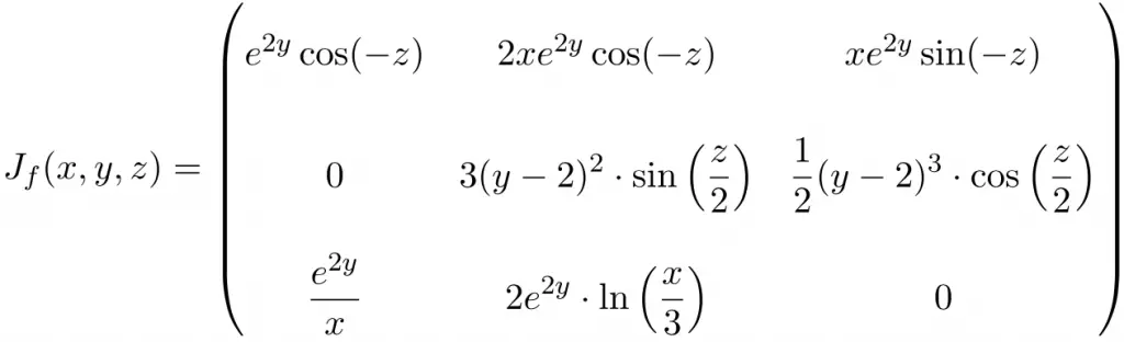
Once we have found the Jacobian matrix, we evaluate it at the point (3,0,π):
![\displaystyle J_f(3,0,\pi)= \begin{pmatrix} \vphantom{\cfrac{\partial f_2}{\partial x}} e^{2\cdot 0}\cos(-\pi) & 2\cdot 3e^{2\cdot 0}\cos(-\pi) & 3e^{2\cdot 0}\sin(-\pi) \\[3ex] \vphantom{\cfrac{\partial f_2}{\partial x}} 0 & \displaystyle 3(0-2)^2\cdot \sin\left(\frac{\pi}{2}\right) & \displaystyle\frac{1}{2}(0-2)^3\cdot \cos\left(\frac{\pi}{2}\right)\\[3ex] \vphantom{\cfrac{\partial f_2}{\partial x}}\displaystyle\frac{e^{2\cdot 0}}{3} &\displaystyle 2e^{2\cdot 0}\cdot \ln\left(\frac{3}{3}\right) & 0\end{pmatrix}](https://www.algebrapracticeproblems.com/wp-content/ql-cache/quicklatex.com-fc83d3ab33b0269bc7589c646d586b9f_l3.svg "Rendered by QuickLaTeX.com")
We calculate all the operations:
![\displaystyle J_f(3,0,\pi)= \begin{pmatrix} \vphantom{\cfrac{\partial f_2}{\partial x}} 1\cdot (-1) & 6\cdot 1\cdot (-1) & 3\cdot 1 \cdot 0 \\[3ex] \vphantom{\cfrac{\partial f_2}{\partial x}} 0 & \displaystyle 3\cdot 4 \cdot 1 & \displaystyle\frac{1}{2}\cdot (-8)\cdot 0\\[3ex] \vphantom{\cfrac{\partial f_2}{\partial x}}\displaystyle\frac{1}{3} &\displaystyle 2\cdot 1\cdot 0 & 0\end{pmatrix}](https://www.algebrapracticeproblems.com/wp-content/ql-cache/quicklatex.com-c62b75e15cecf37f1ed3c37c1a8b7d47_l3.svg "Rendered by QuickLaTeX.com")
And the result of the Jacobian matrix is:
![\displaystyle \bm{J_f(3,0,\pi)=} \begin{pmatrix} \vphantom{\cfrac{\partial f_2}{\partial x}} \bm{-1} & \bm{-6} & \phantom{-}\bm{0} \\[2ex] \bm{0} & \bm{12} & \displaystyle \bm{0} \\[2ex] \displaystyle \frac{\bm{1}}{\bm{3}} &\bm{0}& \bm{0}\end{pmatrix}](https://www.algebrapracticeproblems.com/wp-content/ql-cache/quicklatex.com-a6e712ab2963b500847e83dae0f4922c_l3.svg "Rendered by QuickLaTeX.com")
Jacobian matrix determinant
The determinant of the Jacobian matrix is called the Jacobian determinant, or simply the Jacobian. Note that the Jacobian determinant can only be calculated if the function has the same number of variables as vector components since then the Jacobian matrix is a square matrix.
Jacobian determinant example
Let’s see an example of how to calculate the Jacobian determinant of a function with two variables:

First, we calculate the Jacobian matrix of the function:
![\displaystyle J_f(x,y)=\begin{pmatrix}\cfrac{\phantom{5}\partial f_1}{\partial x}\phantom{5} & \phantom{5}\cfrac{\partial f_1}{\partial y}\phantom{5} \\[3ex] \cfrac{\partial f_2}{\partial x} & \cfrac{\partial f_2}{\partial y}\end{pmatrix} = \begin{pmatrix} \vphantom{\cfrac{\partial f_2}{\partial x}}2x \phantom{5}& -2y \\[2ex] \vphantom{\cfrac{\partial f_2}{\partial x}} 2y & 2x \end{pmatrix}](https://www.algebrapracticeproblems.com/wp-content/ql-cache/quicklatex.com-b2002099d271bf08fa81ba13c1b5b68c_l3.svg "Rendered by QuickLaTeX.com")
And now we take the determinant of the 2×2 matrix:
![\displaystyle \text{det}\bigl(J_f(x,y)\bigr) =\begin{vmatrix} 2x&-2y \\[2ex] 2y & 2x \end{vmatrix} = \bm{4x^2+4y^2}](https://www.algebrapracticeproblems.com/wp-content/ql-cache/quicklatex.com-8c5ec00c9073a80db41250eb7e36f0d4_l3.svg "Rendered by QuickLaTeX.com")
The Jacobian and the invertibility of a function
Now that you have seen the concept of the determinant of the Jacobian matrix, you may be wondering… what is it for?
Well, the Jacobian is used to determine whether a function can be inverted. The inverse function theorem states that if the Jacobian is nonzero, this function is invertible.

Note that this condition is necessary but not sufficient, that is, if the determinant is different from zero we can say that the matrix can be inverted, however, if the determinant is equal to 0 we don’t know whether the function has an inverse or not.
For example, in the example seen before, the determinant Jacobian results in  In that case we can affirm that the function can always be inverted except at the point (0,0), because this point is the only one in which the Jacobian determinant is equal to zero and, therefore, we do not know whether the inverse function exists in this point.
Applications of the Jacobian matrix
In addition to the utility that we have seen of the Jacobian, which determines whether a function is invertible, the Jacobian matrix has other applications.
The Jacobian matrix is used to calculate the critical points of a multivariate function, which are then classified into maximums, minimums, or saddle points using the Hessian matrix. To find the critical points, you have to calculate the Jacobian matrix of the function, set it equal to 0, and solve the resulting equations.

Moreover, another application of the Jacobian matrix is found in the integration of functions with more than one variable, that is, in double, and triple integrals, etc. Since the determinant of the Jacobian matrix allows a change of variable in multiple integrals according to the following formula:


Where T is the variable change function that relates the original variables to the new ones.
Finally, the Jacobian matrix can also be used to compute a linear approximation of any function  around a point

Hessian matrix
What is the Hessian matrix?
The definition of the Hessian matrix is as follows:
The Hessian matrix, or simply Hessian, is an n×n square matrix composed of the second-order partial derivatives of a function of n variables.
The Hessian matrix was named after Ludwig Otto Hesse, a 19th-century German mathematician who made very important contributions to the field of linear algebra.
Thus, the formula for the Hessian matrix is as follows:
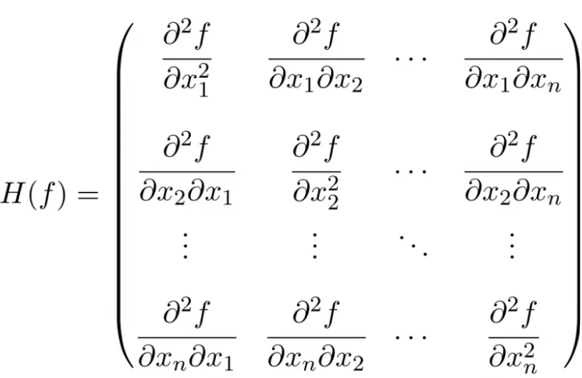
Therefore, the Hessian matrix will always be a square matrix whose dimension will be equal to the number of variables of the function. For example, if the function has 3 variables, the Hessian matrix will be a 3×3 dimension matrix.
Furthermore, Schwarz’s theorem (or Clairaut’s theorem) states that the order of differentiation does not matter, that is, first partially differentiate with respect to the variable  and then with respect to the variable
  is the same as first partially differentiating with respect to and then with respect to

In other words, the Hessian matrix is a symmetric matrix.
Thus, the Hessian matrix is the matrix with the second-order partial derivatives of a function. On the other hand, the matrix with the first-order partial derivatives of a function is the Jacobian matrix.
Hessian matrix example
Once we have seen how to calculate the Hessian matrix, let’s see an example to fully understand the concept:
- Calculate the Hessian matrix at the point (1,0) of the following multivariable function:

First of all, we have to compute the first-order partial derivatives of the function:


Once we know the first derivatives, we calculate all the second-order partial derivatives of the function:


Now we can find the Hessian matrix using the formula for 2×2 matrices:
![\displaystyle H_f (x,y)=\begin{pmatrix}\cfrac{\partial^2 f}{\partial x^2} & \cfrac{\partial^2 f}{\partial x \partial y} \\[4ex] \cfrac{\partial^2 f}{\partial y \partial x} & \cfrac{\partial^2 f}{\partial y^2} \end{pmatrix}](https://www.algebrapracticeproblems.com/wp-content/ql-cache/quicklatex.com-ff3e4c962def29f33dd2f34732f334a5_l3.svg "Rendered by QuickLaTeX.com")
![\displaystyle H_f (x,y)=\begin{pmatrix}6x +6 &-4 \\[2ex] -4 & 12y^2+8 \end{pmatrix}](https://www.algebrapracticeproblems.com/wp-content/ql-cache/quicklatex.com-8c06b3051a44b5efe9f0c34ce264c361_l3.svg "Rendered by QuickLaTeX.com")
So the Hessian matrix evaluated at the point (1,0) is:
![\displaystyle H_f (1,0)=\begin{pmatrix}6\cdot 1 +6 &-4 \\[2ex] -4 & 12\cdot 0^2+8 \end{pmatrix}](https://www.algebrapracticeproblems.com/wp-content/ql-cache/quicklatex.com-eace78fb732987eeb6b43551ae4694e0_l3.svg "Rendered by QuickLaTeX.com")
![\displaystyle H_f (1,0)=\begin{pmatrix}12&-4\\[2ex]-4&8\end{pmatrix}](https://www.algebrapracticeproblems.com/wp-content/ql-cache/quicklatex.com-3e11d47a59625bb384f69f19fe93e351_l3.svg "Rendered by QuickLaTeX.com")
Practice problems on finding the Hessian matrix
Problem 1
Find the Hessian matrix of the following 2 variable function at point (1,1):

Solution
First, we compute the first-order partial derivatives of the function:


Then we calculate all the second-order partial derivatives of the function:


So the Hessian matrix is defined as follows:
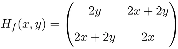
Finally, we evaluate the Hessian matrix at point (1,1):
![\displaystyle H_f (1,1)=\begin{pmatrix}2\cdot 1 &2 \cdot 1+2\cdot 1 \\[1.5ex] 2\cdot 1+2\cdot 1 & 2\cdot 1 \end{pmatrix}](https://www.algebrapracticeproblems.com/wp-content/ql-cache/quicklatex.com-24ec8ef669592d56a978c180e998030d_l3.svg "Rendered by QuickLaTeX.com")
![\displaystyle \bm{H_f (1,1)}=\begin{pmatrix}\bm{2} & \bm{4} \\[1.1ex] \bm{4} & \bm{2} \end{pmatrix}](https://www.algebrapracticeproblems.com/wp-content/ql-cache/quicklatex.com-61df795dcb40314d2bcce4249a38cb05_l3.svg "Rendered by QuickLaTeX.com")
Problem 2
Calculate the Hessian matrix at the point (1,1) of the following function with two variables:

Solution
First, we differentiate the function with respect to x and with respect to y:


Once we have the first derivatives, we calculate the second-order partial derivatives of the function:


So the Hessian matrix of the function is a square matrix of order 2:
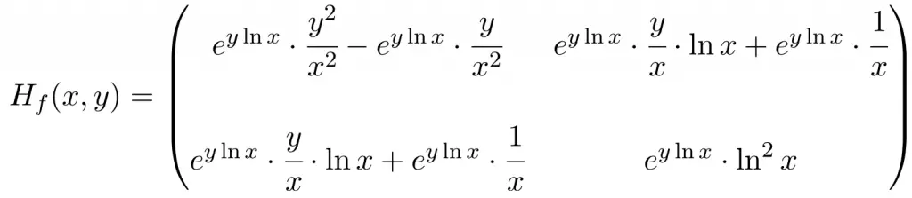
And we evaluate the Hessian matrix at point (1,1):
![\displaystyle H_f (1,1)=\begin{pmatrix} e^{1\ln (1)} \displaystyle \cdot \cfrac{1^2}{1^2} - e^{1\ln (1)} \cdot \cfrac{1}{1^2}& e^{1\ln (1)} \cdot \cfrac{1}{1}\cdot \ln (1) + e^{1\ln (1)}\cdot \cfrac{1}{1} \\[3ex] e^{1\ln (1)} \cdot \cfrac{1}{1}\cdot \ln (1) + e^{1\ln (1)}\cdot \cfrac{1}{1} & e^{1\ln (1)} \cdot \ln ^2 (1) \end{pmatrix}](https://www.algebrapracticeproblems.com/wp-content/ql-cache/quicklatex.com-961d536381ad3f70563c0090795682dc_l3.svg "Rendered by QuickLaTeX.com")
![\displaystyle H_f (1,1)=\begin{pmatrix}e^{0} \cdot 1 - e^{0} \cdot 1& e^{0} \cdot 1\cdot 0 + e^{0}\cdot 1 \\[2ex] e^{0} \cdot 1\cdot 0 + e^{0}\cdot 1 & e^{0} \cdot 0\end{pmatrix}](https://www.algebrapracticeproblems.com/wp-content/ql-cache/quicklatex.com-13018274f5af2c55551d07ded022091c_l3.svg "Rendered by QuickLaTeX.com")
![\displaystyle H_f (1,1)=\begin{pmatrix}1 - 1& 0+ 1 \\[1.5ex] 0 +1 & 1 \cdot 0\end{pmatrix}](https://www.algebrapracticeproblems.com/wp-content/ql-cache/quicklatex.com-b68e9323591b6d1d467521516106f1f8_l3.svg "Rendered by QuickLaTeX.com")
![\displaystyle \bm{H_f (1,1)}=\begin{pmatrix}\bm{0} & \bm{1} \\[1.1ex] \bm{1} & \bm{0} \end{pmatrix}](https://www.algebrapracticeproblems.com/wp-content/ql-cache/quicklatex.com-7f342e023151313f6ac401f28514d65a_l3.svg "Rendered by QuickLaTeX.com")
Problem 3
Compute the Hessian matrix at the point (0,1,π) of the following 3 variable function:

Solution
To compute the Hessian matrix first we have to calculate the first-order partial derivatives of the function:


Once we have computed the first derivatives, we calculate the second-order partial derivatives of the function:


So the Hessian matrix of the function is a square matrix of order 3:
![\displaystyle H_f(x,y,z)=\begin{pmatrix}e^{-x}\cdot \sin(xy) & -ze^{-x}\cdot \cos(yz) &-ye^{-x}\cdot \cos(yz) \\[1.5ex] -ze^{-x}\cdot \cos(yz)&-z^2e^{-x}\cdot \sin(yz) &e^{-x}\cdot \cos(yz)-yze^{-x}\cdot \sin(yz) \\[1.5ex] -ye^{-x}\cdot \cos(yz)& e^{-x}\cdot \cos(yz)-yze^{-x}\cdot \sin(yz)& -y^2e^{-x}\cdot \sin(yz)\end{pmatrix}](https://www.algebrapracticeproblems.com/wp-content/ql-cache/quicklatex.com-8ee22cca8c6ac1aa0afb686fe336974f_l3.svg "Rendered by QuickLaTeX.com")
And finally, we substitute the variables for their respective values at the point (0,1,π):
![\displaystyle H_f(0,1,\pi)=\begin{pmatrix}e^{-0}\cdot \sin(1\pi) & -\pi e^{-0}\cdot \cos(1\pi) &-1e^{-0}\cdot \cos(1\pi) \\[1.5ex] -\pi e^{-0}\cdot \cos(1 \pi)&-\pi^2e^{-0}\cdot \sin(1 \pi) &e^{-0}\cdot \cos(1 \pi)-1 \pi e^{-0}\cdot \sin(1 \pi) \\[1.5ex] -1e^{-0}\cdot \cos(1 \pi)& e^{-0}\cdot \cos(1 \pi)-1 \pi e^{-0}\cdot \sin(1 \pi)& -1^2e^{-0}\cdot \sin(1 \pi) \end{pmatrix}](https://www.algebrapracticeproblems.com/wp-content/ql-cache/quicklatex.com-0bcac084f40db6c0363ca40eef2fbb14_l3.svg "Rendered by QuickLaTeX.com")
![\displaystyle H_f(0,1,\pi)=\begin{pmatrix}1\cdot 0 & -\pi \cdot 1 \cdot (-1)&-1\cdot 1 \cdot (-1) \\[1.5ex] -\pi \cdot 1 \cdot (-1) &-\pi^2\cdot 1\cdot 0 &1 \cdot (-1)-\pi \cdot 1\cdot 0 \\[1.5ex] -1\cdot 1 \cdot (-1) & 1\cdot (-1) - \pi \cdot 1\cdot 0 & -1\cdot 1 \cdot 0 \end{pmatrix}](https://www.algebrapracticeproblems.com/wp-content/ql-cache/quicklatex.com-0594cf258bfcfbde5f12045a3b9a4603_l3.svg "Rendered by QuickLaTeX.com")
![\displaystyle \bm{H_f(0,1,\pi)=}\begin{pmatrix}\bm{0}&\bm{\pi}&\bm{1}\\[1.5ex]\bm{\pi}&\bm{0}&\bm{-1}\\[1.5ex]\bm{1}&\bm{-1}&\bm{0}\end{pmatrix}](https://www.algebrapracticeproblems.com/wp-content/ql-cache/quicklatex.com-40cd7c1b2da5d7b520b900fc0760b463_l3.svg "Rendered by QuickLaTeX.com")
Problem 4
Determine the Hessian matrix at the point (2, -1, 1, -1) of the following function with 4 variables:

Solution
The first step is to find the first-order partial derivatives of the function:


Now we solve the second-order partial derivatives of the function:


So the expression of the 4×4 Hessian matrix obtained by solving all the partial derivatives is the following:
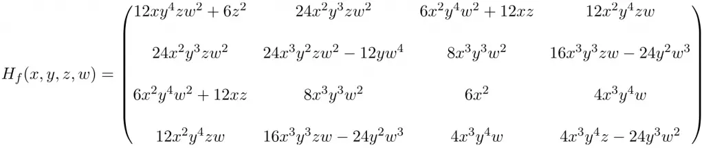
And finally, we substitute the unknowns for their respective values of the point (2, -1, 1, -1) and perform the calculations:
![\displaystyle \bm{H_f(2,-1,1,-1)=}\begin{pmatrix}\bm{30}&\bm{-96}&\bm{48}&\bm{-48}\\[1.5ex]\bm{-96}&\bm{204}&\bm{-64}&\bm{152}\\[1.5ex]\bm{48}&\bm{-64}&\bm{24}&\bm{-32}\\[1.5ex]\bm{-48}&\bm{152}&\bm{-32}&\bm{56}\end{pmatrix}](https://www.algebrapracticeproblems.com/wp-content/ql-cache/quicklatex.com-f5081444517d11824573343b3d558bdf_l3.svg "Rendered by QuickLaTeX.com")
Applications of the Hessian matrix
You may be wondering… what is the Hessian matrix for? Well, the Hessian matrix has several applications in mathematics. Next, we will see what the Hessian matrix is used for.
Minimum, maximum, or saddle point
If the gradient of a function is zero at some point, that is f(x)=0, then function f has a critical point at x. In this regard, we can determine whether that critical point is a local minimum, a local maximum, or a saddle point using the Hessian matrix:
- If the Hessian matrix is positive definite (all the eigenvalues of the Hessian matrix are positive), the critical point is a local minimum of the function.
- If the Hessian matrix is negative definite (all the eigenvalues of the Hessian matrix are negative), the critical point is a local maximum of the function.
- If the Hessian matrix is indefinite (the Hessian matrix has positive and negative eigenvalues), the critical point is a saddle point.
Note that if an eigenvalue of the Hessian matrix is 0, we cannot know whether the critical point is an extremum or a saddle point.
Convexity or concavity
Another utility of the Hessian matrix is to know whether a function is concave or convex. And this can be determined by applying the following theorem.
Let  be an open set and
  a function whose second derivatives are continuous, its concavity or convexity is defined by the Hessian matrix:
- Function f is convex on set A if, and only if, its Hessian matrix is positive semidefinite at all points on the set.
- Function f is strictly convex on set A if, and only if, its Hessian matrix is positive definite at all points on the set.
- Function f is concave on set A if, and only if, its Hessian matrix is negative semi-definite at all points on the set.
- Function f is strictly concave on set A if, and only if, its Hessian matrix is negative definite at all points on the set.
Taylor polynomial
The expansion of the Taylor polynomial for functions of 2 or more variables at the point  begins as follows:

As you can see, the second-order terms of the Taylor expansion are given by the Hessian matrix evaluated at point  This application of the Hessian matrix is very useful in large optimization problems.
Bordered Hessian matrix
Another use of the Hessian matrix is to calculate the minimum and maximum of a multivariate function  restricted to another function
  To solve this problem, we use the bordered Hessian matrix, which is calculated by applying the following steps:
Step 1: Calculate the Lagrange function, which is defined by the following expression:

Step 2: Find the critical points of the Lagrange function. To do this, we calculate the gradient of the Lagrange function, set the equations equal to 0, and solve the equations.


Step 3: For each point found, calculate the bordered Hessian matrix, which is defined by the following formula:
![\displaystyle H(f,g) = \begin{pmatrix}0 & \cfrac{\partial g}{\partial x_1} & \cfrac{\partial g}{\partial x_2} & \cdots & \cfrac{\partial g}{\partial x_n} \\[4ex] \cfrac{\partial g}{\partial x_1} & \cfrac{\partial^2 f}{\partial x_1^2} & \cfrac{\partial^2 f}{\partial x_1\,\partial x_2} & \cdots & \cfrac{\partial^2 f}{\partial x_1\,\partial x_n} \\[4ex] \cfrac{\partial g}{\partial x_2} & \cfrac{\partial^2 f}{\partial x_2\,\partial x_1} & \cfrac{\partial^2 f}{\partial x_2^2} & \cdots & \cfrac{\partial^2 f}{\partial x_2\,\partial x_n} \\[3ex] \vdots & \vdots & \vdots & \ddots & \vdots \\[3ex] \cfrac{\partial g}{\partial x_n} & \cfrac{\partial^2 f}{\partial x_n\,\partial x_1} & \cfrac{\partial^2 f}{\partial x_n\,\partial x_2} & \cdots & \cfrac{\partial^2 f}{\partial x_n^2}\end{pmatrix}](https://www.algebrapracticeproblems.com/wp-content/ql-cache/quicklatex.com-1b61659a618df49922042741597aa22d_l3.svg "Rendered by QuickLaTeX.com")
Step 4: Determine for each critical point whether it is a maximum or a minimum:
- The critical point will be a local maximum of function under the restrictions of function
 if the last n-m (where n is the number of variables and m is the number of constraints) major minors of the bordered Hessian matrix evaluated at the critical point have alternating signs starting with the negative sign.
 - The critical point will be a local minimum of function under the restrictions of function if the last n-m (where n is the number of variables and m is the number of constraints) major minors of the bordered Hessian matrix evaluated at the critical point all have negative signs.
Note that the local minimums or maximums of a restricted function do not have to be that of the unrestricted function. So the bordered Hessian matrix only works for this type of problem.
Source:
https://www.algebrapracticeproblems.com/hessian-matrix/
https://www.algebrapracticeproblems.com/jacobian-matrix-determinant/