REINFORCE Algorithm explained in Policy-Gradient based methods with Python Code
2021-03-01Python Scipy sparse matrices explained
2021-04-28Handling cyclical features, such as hours in a day, for machine learning pipelines with Python example

What’s the difference between 23 and 1? If we’re talking about time, it’s 2.
Hours of the day, days of the week, months in a year, and wind direction are all examples of features that are cyclical. Many new machine learning engineers don’t think to convert these features into a representation that can preserve information such as hour 23 and hour 0 being close to each other and not far.
A cyclical variable is a fancy name for a feature that repeats cyclically. It’s vital to ensure a model interprets cyclical features correctly as the two-hour difference between 23 and 1 would otherwise be interpreted as -22. In this blog post, I’ll explore this feature engineering task and see if it really improves the predictive capability of a simple model.
Types of Cyclical Variables
Wind direction, seasons, time, and days (of a month, year, etc.) are all cyclical variables. A more general rule of thumb is anything is cyclical in real life (wind direction), repeats (seasons), or has an important denominator (days of a month or year). Categorical and continuous cyclical features can be treated similarly.
The Cyclical Formula
Here’s the general formula to convert a variable into a set of cyclical features:
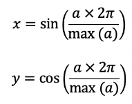
Note that this will mean creating two features.
Examples
We’ll look at two examples; how this formula works with analog clocks and then at the more practical application of wind direction.
Let’s look at a 12-hour clock at precisely 6 o’clock (unlike the clock above).
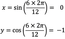
max(a) is 12 as you can’t have a number higher than 12 on your typical clock. It’s important to note that 12:01 am is the same as 00:01, which needs to be taken into account with other cyclical features. If max(a) isn’t the same as 0, then add 1 to the max (see below with the wind example).
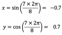
Now let’s say my apartment has a north-facing window that I keep open and I want a predictive model for how cold my house will be when I get home. My data shows that a northerly wind will make it cold, and so will a northeasterly, whereas a southerly wind will have no effect. If we number the features 0 to 7, a model will treat higher numbers as having less of an impact based on this data.
But happens when there’s a northwesterly? Intuitively, this would also make my house cold. That’s why we need to capture the cyclical nature of the feature!
Northwesterly Wind
Northerly Wind
Let’s Code!
Dataset introduction and loading
We need a dataset with some date or other cyclical attributes — that’s obvious. A quick Kaggle search resulted in this Hourly Energy Consumption dataset, of which we’ll use the first AEP_hourly.csv file. It’s a couple of MB in size, so download it to your machine.
The first couple of rows look like this, once loaded with Pandas:
import pandas as pd

df = pd.read_csv('data/AEP_hourly.csv.zip')
df.head()
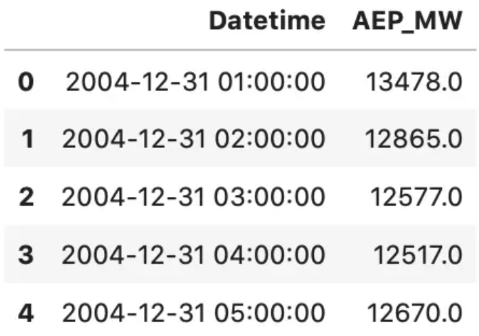
Great — we have some date information, but is it an actual date or a string?
df.dtypes
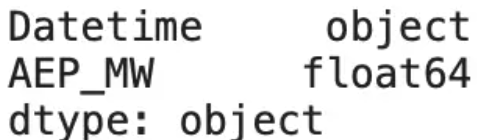
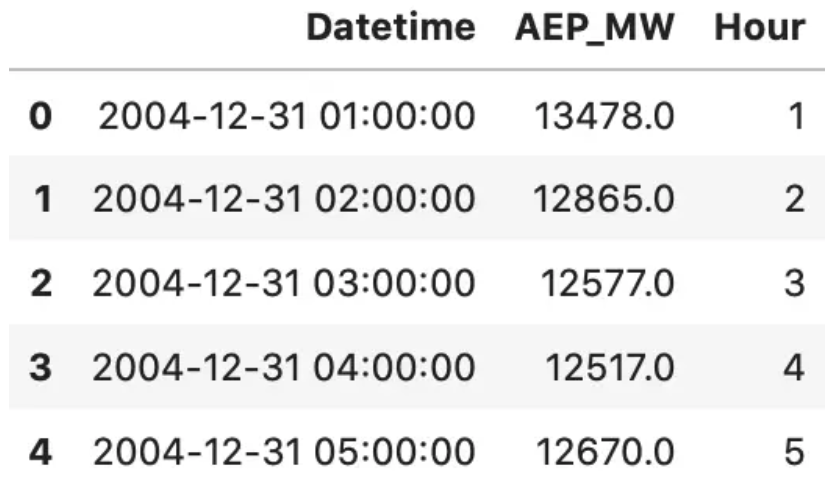
Just as expected, so let’s make a conversion. We’ll also extract the hour information from the date, as that’s what we’re dealing with.
df['Datetime'] = pd.to_datetime(df['Datetime'])
df['Hour'] = df['Datetime'].dt.hour

df.head()
Things are much better now. Let’s isolate the last week’s worth of data (the last 168 records) to visualize why one-hot encoding isn’t a good thing to do.
last_week = df.iloc[-168:]
import matplotlib.pyplot as plt

plt.title('Individual hours', size=20)
plt.plot(range(len(last_week)), last_week['Hour'])
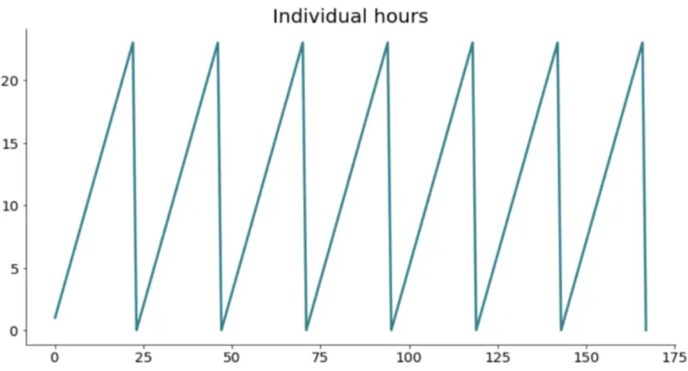
Expected behavior. It’s a cycle that repeats seven times (7 days), and there’s a rough cut-off every day after the 23rd hour. I think you can easily reason why this type of behavior isn’t optimal for cyclical data.
But what can we do about it? Luckily, a lot.
Encoding cyclical data
One-hot encoding wouldn’t be that wise of a thing to do in this case. We’d end up with 23 additional attributes (n — 1), which is terrible for two reasons:
- Massive jump in dimensionality — from 2 to 24
- No connectivity between attributes — hour 23 doesn’t know it’s followed by hour 0
So, what can we do?
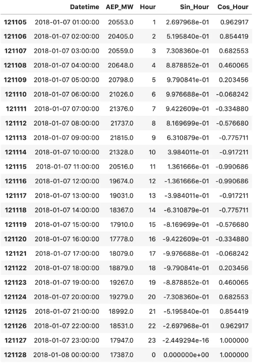
Use sine and cosine transformations. Here are the formulas we’ll use:
Or, in Python:
import numpy as np
last_week['Sin_Hour'] = np.sin(2 * np.pi * last_week['Hour'] / max(last_week['Hour']))
last_week['Cos_Hour'] = np.cos(2 * np.pi * last_week['Hour'] / max(last_week['Hour']))
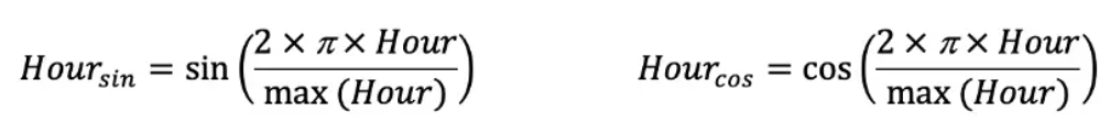
Awesome! Here’s how the last week of data now looks:
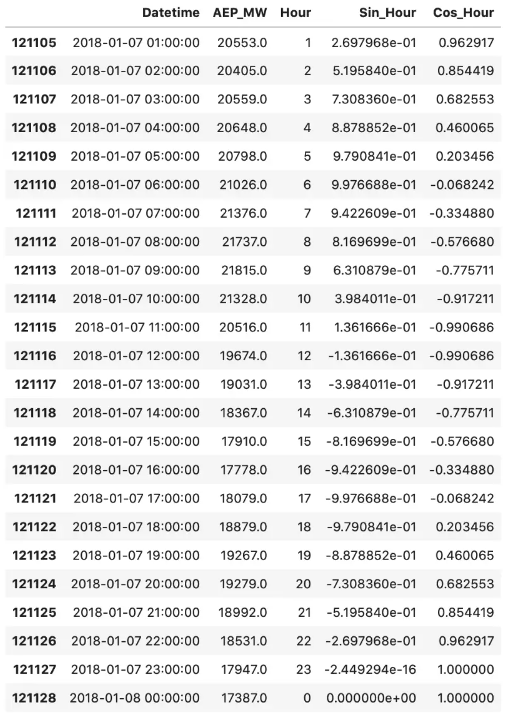
These transformations allowed us to represent time data in a more meaningful and compact way. Just take a look at the last two rows. Sine values are almost identical, but still a bit different. The same goes for every following hour, as it now follows a waveform.
That’s great, but why do we need both functions?
Let’s explore the functions graphically before I give you the answer.
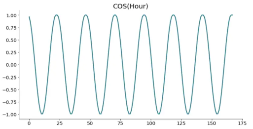
Look at one graph at a time. There’s a problem. The values repeat. Just take a look at the sine function, somewhere between 24 and 48, on the x-axis. If you were to draw a straight line, it would intersect with two points on the same day. That’s not the behavior we want.
To further prove this point, here’s what happens if we draw a scatter plot of both sine and cosine columns:
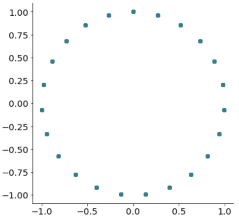
That’s right; we get a perfect cycle. It only makes sense to represent cyclical data with a cycle, don’t you agree?
Examine the Cyclical Encoding effect on the ML pipeline performance
To begin, let’s download a public dataset that has some cyclical qualities. I found a bicycle-sharing dataset online (pardon the double entendre) which includes some basic features, with the aim of predicting how many bikes are being used at any given hour. Let’s download, unzip, and have a quick look.
!curl -O 'https://archive.ics.uci.edu/ml/machine-learning-databases/00275/Bike-Sharing-Dataset.zip'
!mkdir 'data/bike_sharing/'
!unzip 'Bike-Sharing-Dataset.zip' -d 'data/bike_sharing'
  % Total    % Received % Xferd  Average Speed   Time    Time     Time  Current
                                 Dload  Upload   Total   Spent    Left  Speed
100  273k  100  273k    0     0   185k      0  0:00:01  0:00:01 --:--:--  210k
Archive:  Bike-Sharing-Dataset.zip
  inflating: data/bike_sharing/Readme.txt
  inflating: data/bike_sharing/day.csv
  inflating: data/bike_sharing/hour.csv
import pandas as pd

df = pd.read_csv('data/bike_sharing/hour.csv')
print (df.columns.values)
# output
# ['instant' 'dteday' 'season' 'yr' 'mnth' 'hr' 'holiday' 'weekday' 'workingday' 'weathersit' 'temp' 'atemp' 'hum' 'windspeed' 'casual'  'registered' 'cnt']
It looks like there are a bunch of features in here that are likely valuable to predict cnt, the count of users riding bikes (probably the sum of “casual” riders and “registered” riders). Let’s have a look at the mnth (month) feature, and the hr (hour) feature and try to transform them.
df = df[['mnth','hr','cnt']].copy()
print ('Unique values of month:', df.mnth.unique())
print ('Unique values of hour:', df.hr.unique())
# output
# Unique values of month: [ 1  2  3  4  5  6  7  8  9 10 11 12]
# Unique values of hour: [ 0  1  2  3  4  5  6  7  8  9 10 11 12 13 14 15 16 17 18 19 20 21 22 23]
So far, so logical. Months are numbered one through twelve, and hours are numbered 0 through 23.
The Magic
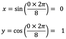
Now the magic happens. We map each cyclical variable onto a circle such that the lowest value for that variable appears right next to the largest value. We compute the x and y components of that point using sin and cos trigonometric functions. You remember your unit circle, right? Here’s what it looks like for the “hours” variable. Zero (midnight) is on the right, and the hours increase counterclockwise around the circle. In this way, 23:59 is very close to 00:00, as it should be.
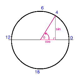
Note that when we perform this transformation for the “month” variable, we also shift the values down by one such that it extends from 0 to 11, for convenience.
import numpy as np

df['hr_sin'] = np.sin(df.hr*(2.*np.pi/24))
df['hr_cos'] = np.cos(df.hr*(2.*np.pi/24))
df['mnth_sin'] = np.sin((df.mnth-1)*(2.*np.pi/12))
df['mnth_cos'] = np.cos((df.mnth-1)*(2.*np.pi/12))
Now instead of hours extending from 0 to 23, we have two new features “hr_sin” and “hr_cos” which each extend from 0 to 1 and combine to have the nice cyclical characteristics we’re after.
The claim is that using this transformation will improve the predictive performance of our models. Let’s give it a shot!
Impact on Model Performance
To begin, let’s try to use just the nominal hours and month features to predict the number of bikes being ridden. I’ll use a basic sklearn neural network and see how well it performs with K-fold cross-validation. The loss function I’ll use is (negative) mean squared error. I’ll also use a standard scaler in a Scikit-Learn Pipeline, though it probably isn’t necessary given the range in values of our two features.
from sklearn.preprocessing import StandardScaler
from sklearn.neural_network import MLPRegressor
from sklearn.pipeline import Pipeline

# Construct the pipeline with a standard scaler and a small neural network
estimators = []
estimators.append(('standardize', StandardScaler()))
estimators.append(('nn', MLPRegressor(hidden_layer_sizes=(5,), max_iter=1000)))
model = Pipeline(estimators)

# To begin, let's use only these two features to predict 'cnt' (bicycle count)
features = ['mnth','hr']
X = df[features].values
y = df.cnt

# We'll use 5-fold cross validation. That is, a random 80% of the data will be used
# to train the model, and the prediction score will be computed on the remaining 20%.
# This process is repeated five times such that the training sets in each "fold"
# are mutually orthogonal.
from sklearn.model_selection import KFold
from sklearn.model_selection import cross_val_score
kfold = KFold(n_splits=5)

results = cross_val_score(model, X, y, cv=kfold, scoring='neg_mean_squared_error')
print ('CV Scoring Result: mean=', np.mean(results), 'std=', np.std(results))

# output
# CV Scoring Result: mean= -31417.4341504 std= 12593.3781285
That’s a pretty large average MSE, but that’s the point. The neural network struggles to interpret month and hour features because they aren’t represented in a logical (cyclical) way. These features are more categorical than numerical, which is a problem for the network.
Let’s repeat the same exercise, but using the four newly engineered features we created above.
features = ['mnth_sin', 'mnth_cos', 'hr_sin', 'hr_cos']
X = df[features].values

results = cross_val_score(model, X, y, cv=kfold, scoring='neg_mean_squared_error')
print ('CV Scoring Result: mean=', np.mean(results), 'std=', np.std(results))
# output
# CV Scoring Result: mean= -23702.9269968 std= 9942.45888087
Success! The average MSE improved by almost 25% (remember this is negative MSE so the closer to zero the better)!
To be clear, I’m not saying that this model will do a good job at predicting the number of bikes being ridden but taking this feature engineering step for the cyclical features definitely helped. The model had an easier time interpreting the engineered features. What’s nice is that this feature engineering method not only improves performance, but it does it in a logical way that humans can understand. I’ll definitely be employing this technique in my future analyses, and I hope you do too.
References:
http://blog.davidkaleko.com/feature-engineering-cyclical-features.html
https://www.thedataschool.com.au/ryan-edwards/feature-engineering-cyclical-variables/
https://betterdatascience.com/cyclical-data-machine-learning/
https://www.kaggle.com/code/avanwyk/encoding-cyclical-features-for-deep-learning/notebook
https://ianlondon.github.io/blog/encoding-cyclical-features-24hour-time/